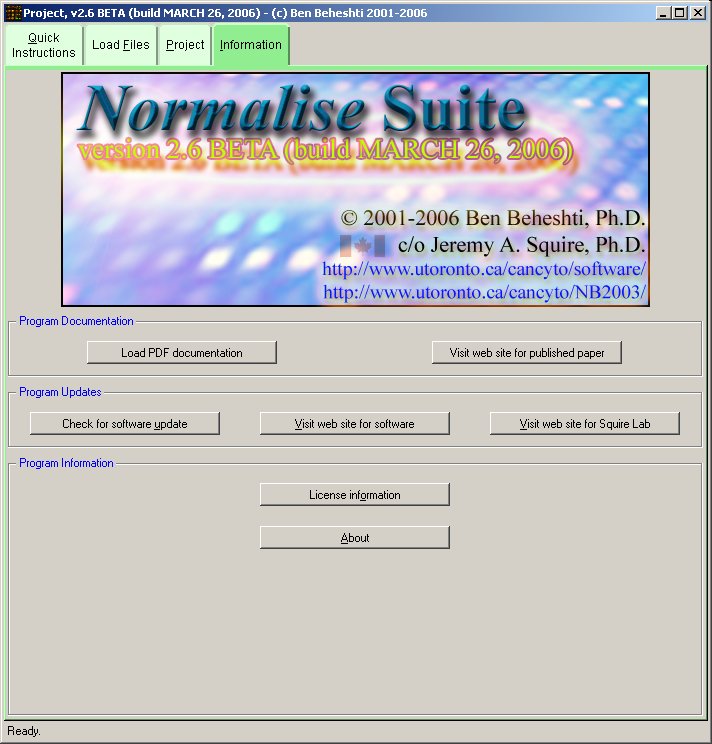
- This software may be cited as indicated below.
This software suite is free for academic, non-commercial use. Use of the software suite by businesses, or for commercial purposes, requires separate permission and/or a license to be purchased directly from the Squire Lab.
- Genelist Importer
This initial step may be necessary to allow the software suite to support your microarray.
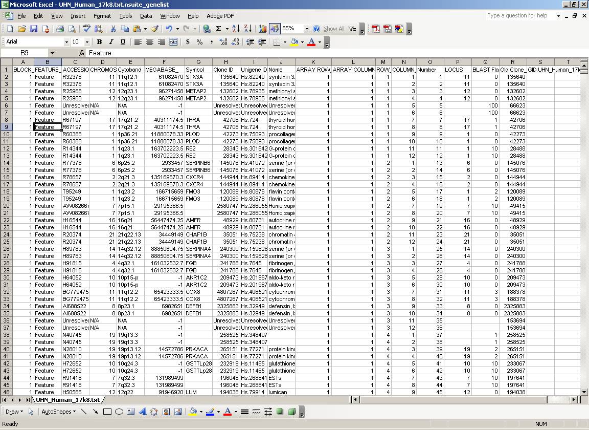
A "genelist" is a text file containing information about the gene identity, spotting organization, and sometimes chromosomal localization of the features (spots) of the microarray. As there is no common format for genelists of microarray products from different sources, Genelist Importer is used to prepare the genelists for the experiments you are going to analyse into a standardized format that the software suite can understand (prior to analysing your microarray experiments).
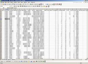
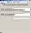
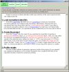
The structure of the genelist is a tab-delimited text formatted file, and should have at a minimum the GRID/BLOCK, ROW, COLUMN, and ACCESSION/ID information for each feature on the array. Optional information may include CHROMOSOME and MEGABASE information. The following figure shows a representative genelist (after importing) (click image to enlarge):
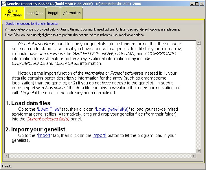
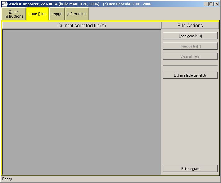
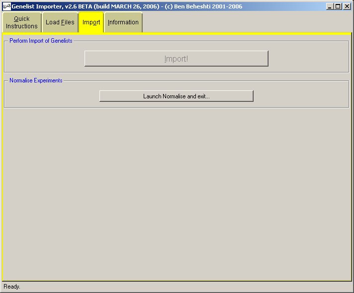
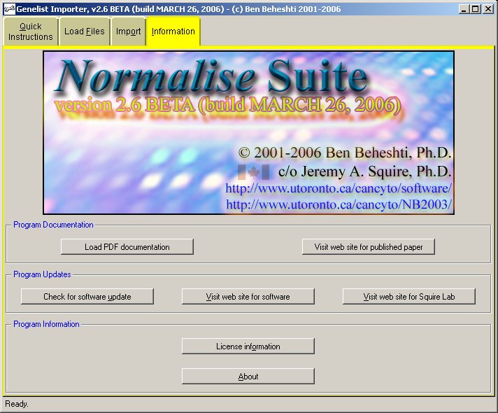
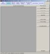
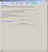
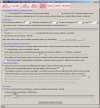
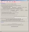
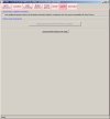
For convenience, some commonly used genelists are already preconfigured (imported) for you, and packaged with the software. This includes most of the UHN microarrays, BCCA SMRT microarrays, and Spectral Genomics microarrays. The images below show the Genelist Importer software user interface (click images to enlarge):

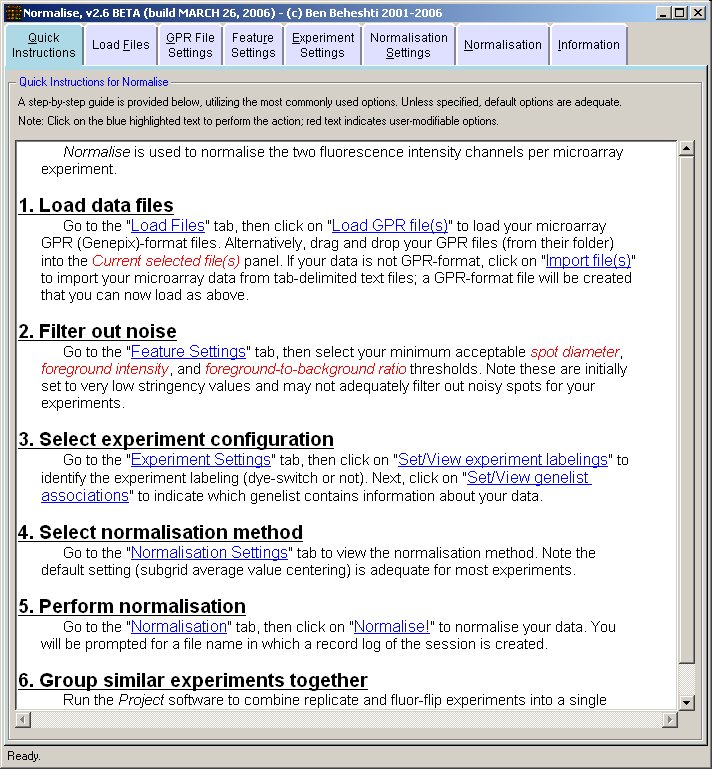
- Normalise
This is the first step in the analysis of your microarray data.
Normalise is used to mathematically equalize (by average value centering) the two fluorescence intensity channels per microarray experiment to facilitate data analysis. Technically, this equalization is necessary to account for experimental differences (eg. DNA labeling, hybridization efficiency) between the two samples that would lead to incorrect results. Furthermore, it can help to correct for areas of signal noise on the microarray present within one (or both) channels.
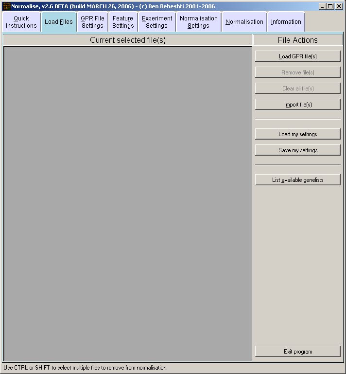
Normalise recognizes GenePix (GPR) format data files, or users may directly import microarray non-normalised data ( tab-delimited text format) produced by their microarray scanner software.
Load any or all of your GPR files into Normalise to be normalised, including replicates, dye-switches, etc. Note you may normalise different data files of different experiments/samples at the same time, as each data file is normalised independently of the others.
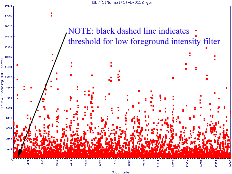
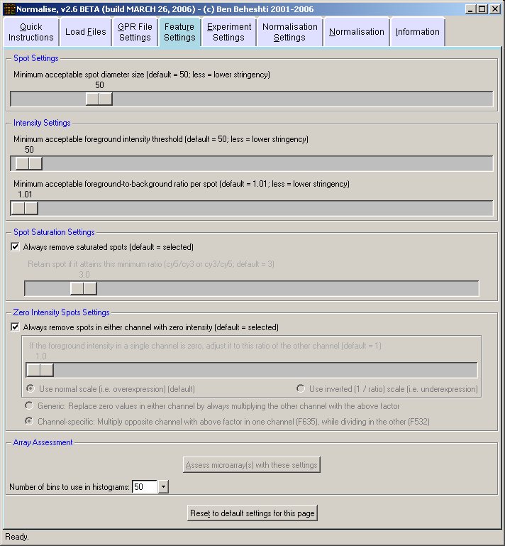
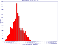
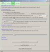
Filters may be applied to remove noisy or outlier features, with adjustable threshold settings based on foreground intensity level, foreground-to-background intensity ratio, saturation level, spot diameter size, and zero intensity values. Prior to normalisation, the software can generate histograms of intensity distributions of each channel. This information may be used for setting the filters (click images to enlarge):

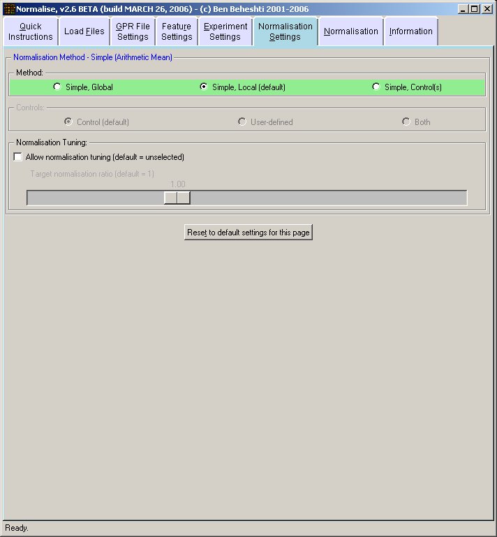
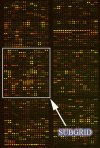
Generally, microarrays are printed with features in subgroups (subgrids) along the glass slide. The software allows for microarray data to be normalised across the entire array ("global"), or by individual subgrids ("local"). The benefit of subgrid normalisation (versus entire array normalisation) is its robustness, as one region of the microarray is not affected by noise in another.
The following image demonstrates features spotted into subgrids on a microarray (click on image to enlarge):
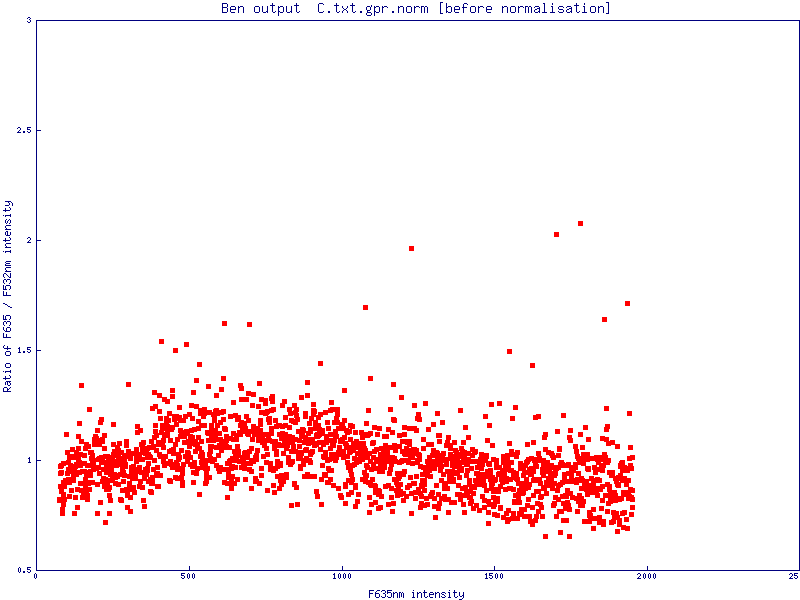
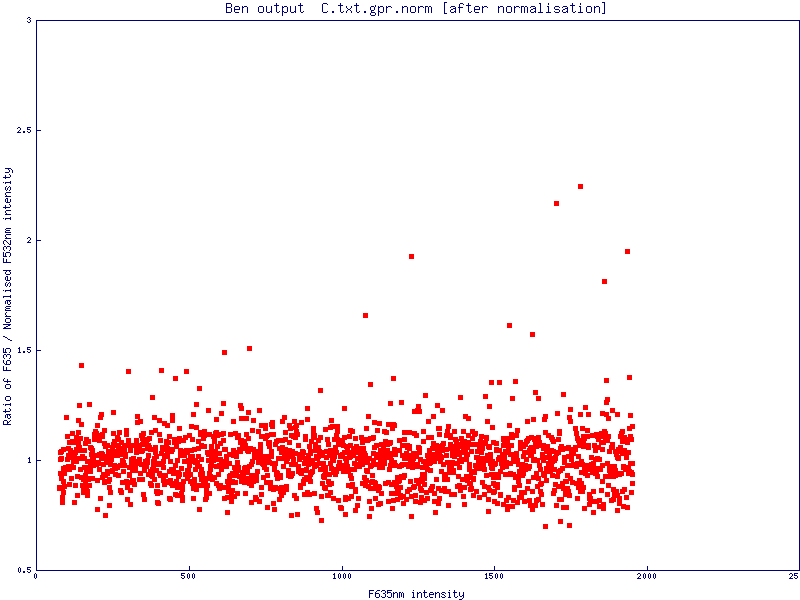
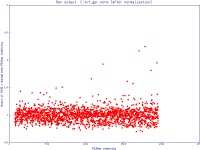
The simple scatter plot images below are generated by Normalise to demonstrate the effects of normalisation (pre- and post-) on a data set (click images to enlarge):

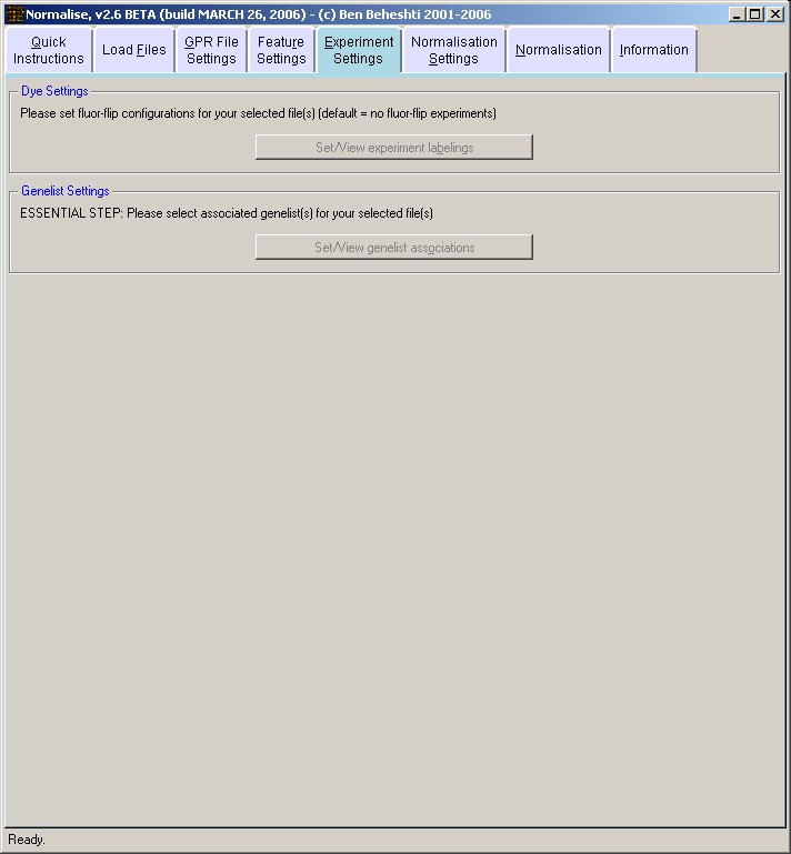
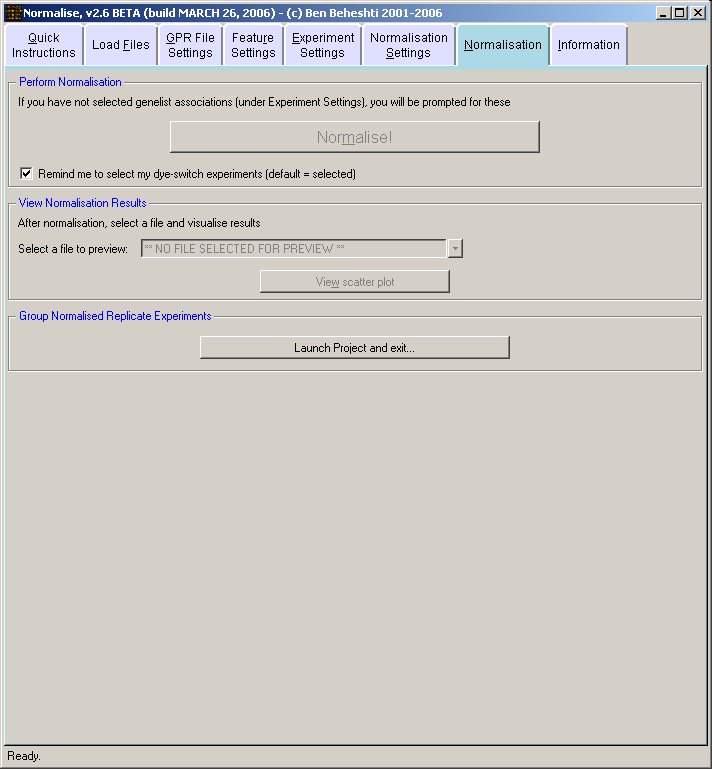
Note: The most commonly used settings are selected by default.
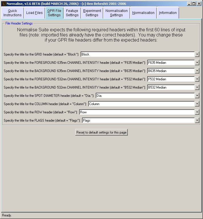
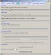
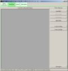
The images below show the Normalise software user interface (click images to enlarge):


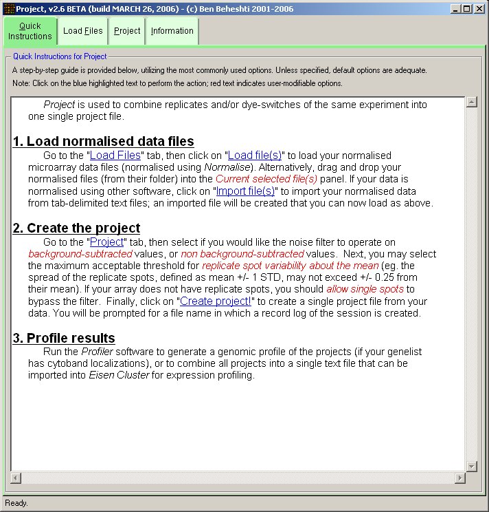
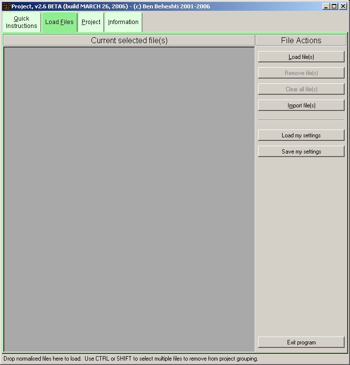
- Project
This is the second step in the analysis of your microarray data.
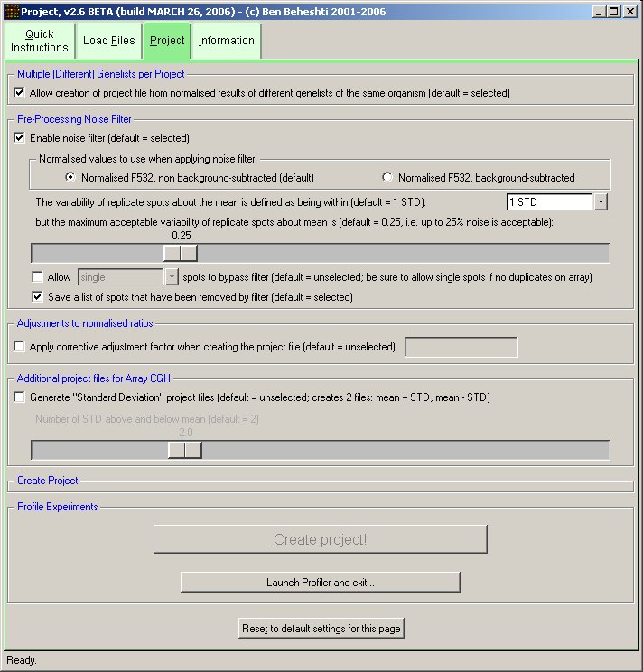
Project is used to combine normalised replicates and/or dye-switches of the same experiment into one single project file. Thus, for each feature there is a single averaged intensity ratio. Alternatively, one can create separate project files per each of the replicate (or dye-switch) experiments of a sample, to enable one to view the profiles of each experiment separately.
The software loads normalised microarray data (created by Normalise); however, users may directly import their own custom normalised microarray data ( tab-delimited text format). Load into Project only the normalised files from the experiments (of a sample) that are to be combined; do not mix different experiment samples (unless you intended to do this for any reason).
A filter may be applied to remove noisy features before combining experiments into a single project. For instance, many microarray features are printed in duplicate on a single slide. By combining two normalised experiments of the same sample (replicate or dye-switch), there are 4 data points. One may specify a filter such that the spread of these spots may not exceed +/- 0.25 from their mean.
Note: The most commonly used settings are selected by default.
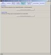
The images below show the Project software user interface (click images to enlarge):
- Profiler
This is the final step in the profiling your microarray (CGH) data.
Profiler loads project files (created by Project) and is used to create genomic profiles of your microarray CGH (or expression) experiments. Profiler can also perform data smoothing of the data as well as automatic delineation of regions of copy number change in the microarray experiment(s).
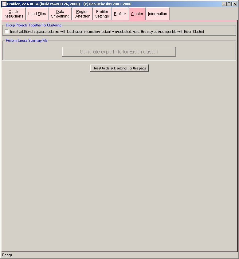
Additionally, Profiler may be used to create a composite text file of your microarray results (CGH or expression) that can be imported into Eisen Cluster for hierarchical clustering or other bioinformatics analyses. Load into Profiler only the project file(s) from the experiments that are to be plotted. It is possible to profile as many or as few projects into a single plot as desired.
- Data Smoothing:
Data smoothing may be applied to the chromosome profiles to reduce experimental noise while emphasizing consistent imbalances along each chromosome.
Profiler uses a built-in sliding window data smoother algorithm that can utilize median, average, or locally weighted scatter plot smoother ( LOWESS; for review, see PDF) methods.
The image below uses LOWESS data smoothing on a very noisy sample (microarray CGH on paraffin-embedded tissue), demonstrating the effects of varying window size on data smoothing (click image to enlarge):
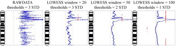
Below is another example of LOWESS data smoothing in a whole genome plot (x-axis: chromosome 1ptel to the left, down to Xqtel to the right). This image cycles from 0 smoothing (raw plot) through to excessive smoothing to show the effects of different window sizes.
With a smaller window, there is more fidelity with the original data, yet noise persists. With a larger window, the curve is smoother although artefactual data is introduced. The key is to find the right balance (click image to enlarge):
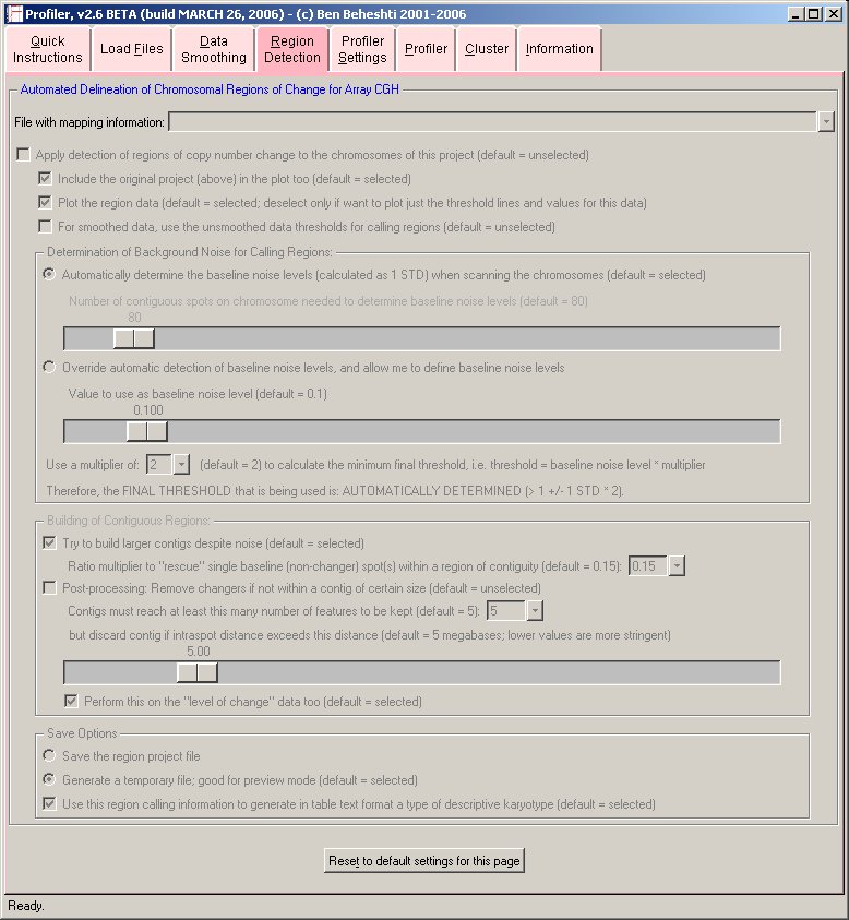
- Region Detection:
Automated region calling may be applied to the chromosome profiles to allow one to identify regions of copy number gain and loss in the data.
In determining the thresholds for gain and loss, two methods are available to the user: 1) user-defined thresholds; or 2) allowing the software to automatically determine the thresholds based on baseline noise determination within the experiment, using a sliding window algorithm, described as follows:
Automated region detection using a sliding window algorithm:
BACKGROUND: Ideally, a normal vs. normal microarray CGH experiment should allow one to define the experimental baseline noise level to use as thresholds for defining copy number change. However, intraexperimental variation (introduced by differences in hybridization, labeling, and scanning) precludes one from using baseline noise levels determined from one experiment, and applying to another experiment. To circumvent this, a sliding window algorithm was developed.
HYPOTHESIS: When performing microarray CGH on a sample with no copy number changes, the baseline noise level would simply be calculated as the standard deviation (i.e. variability) of all the spots across the genome. However, in samples with copy number alterations (eg. tumour samples), determination of baseline noise by this method would be biased, as the calculated standard deviation would be larger than expected (due to contribution of spots in regions of copy number alteration). Instead, by using a method of sampling many areas of the genome, determining the variability in those samplings, and identifying the minimum calculated variability of all those samplings, one may obtain a more representative value of the baseline noise. Finally, rather than randomly sampling across the genome, a sliding window method (of user-defined window size) may be used to systematically calculate the variability across all possible samplings in the genome. This derived minimum variability may thus be used as the noise threshold for determining copy number changes.
ALGORITHM: The window is defined as a number of contiguous linear array spots along each chromosome (default window size = 80). Starting at the pter of a chromosome (usually, chromosome 1), the window is populated with normalized intensity ratios. Subsequently, the standard deviation (i.e. variability) of the window is determined. The window subsequently slides a single spot position toward the chromosome qter, and repeats the variability determination for the new window. This process is reiterated until the end of the chromosome is reached. The window then moves to the next chromosome and repeats this process. When the entire genome has been examined, the baseline noise threshold is determined to be the minimum calculated variability sampled from across the entire genome. This threshold is then used in determining which spots have copy number imbalance. Note chromosomes with number of contiguous features less than the window size are currently excluded.
Please note: The default size of the sliding window was determined by comparisons between metaphase CGH and array CGH results performed in this laboratory using NUB-7, prostate, and other cell lines with established genomic imbalance data to derive empirical threshold values for a given array experiment. Users of the software should empirically derive their own optimal window size. In the future, the software will allow for automatic determination of optimal window size based on statistical analysis of the raw data.
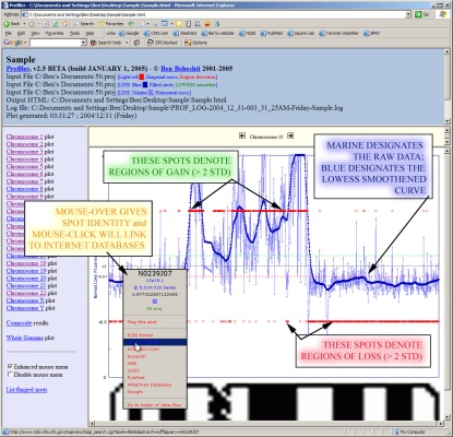
Below is an example of results from automated region calling. The blue line represents the raw data; the green line is data smoothening of the raw data; and the
red points delineate regions of copy number change from the data smoothened results (using thresholds derived from the raw data).
Lines indicating thresholds (green for gain; red for loss) are included on the plot. The image below demonstrates the effects of using different window sizes in region calling (click image to enlarge):
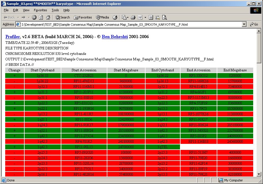
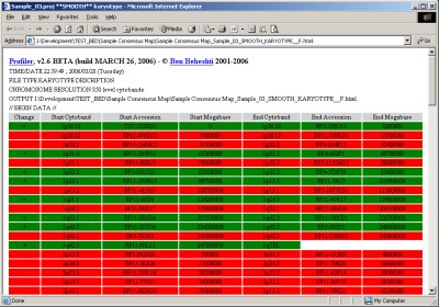
Automated region detection and consensus regions determination for experiments are automatically provided with a pseudo-karyotype description (click image to enlarge):
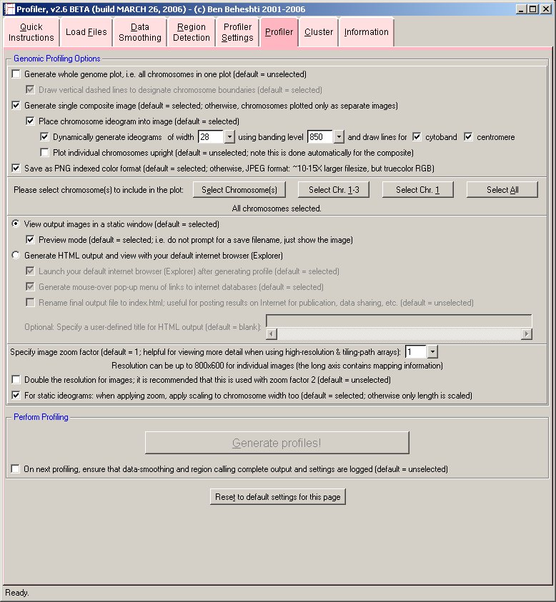
- Profiling:
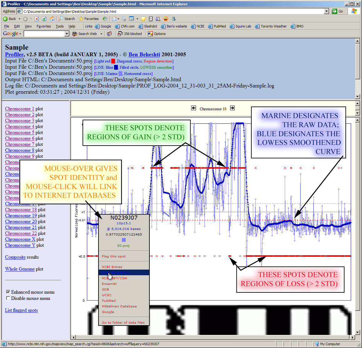
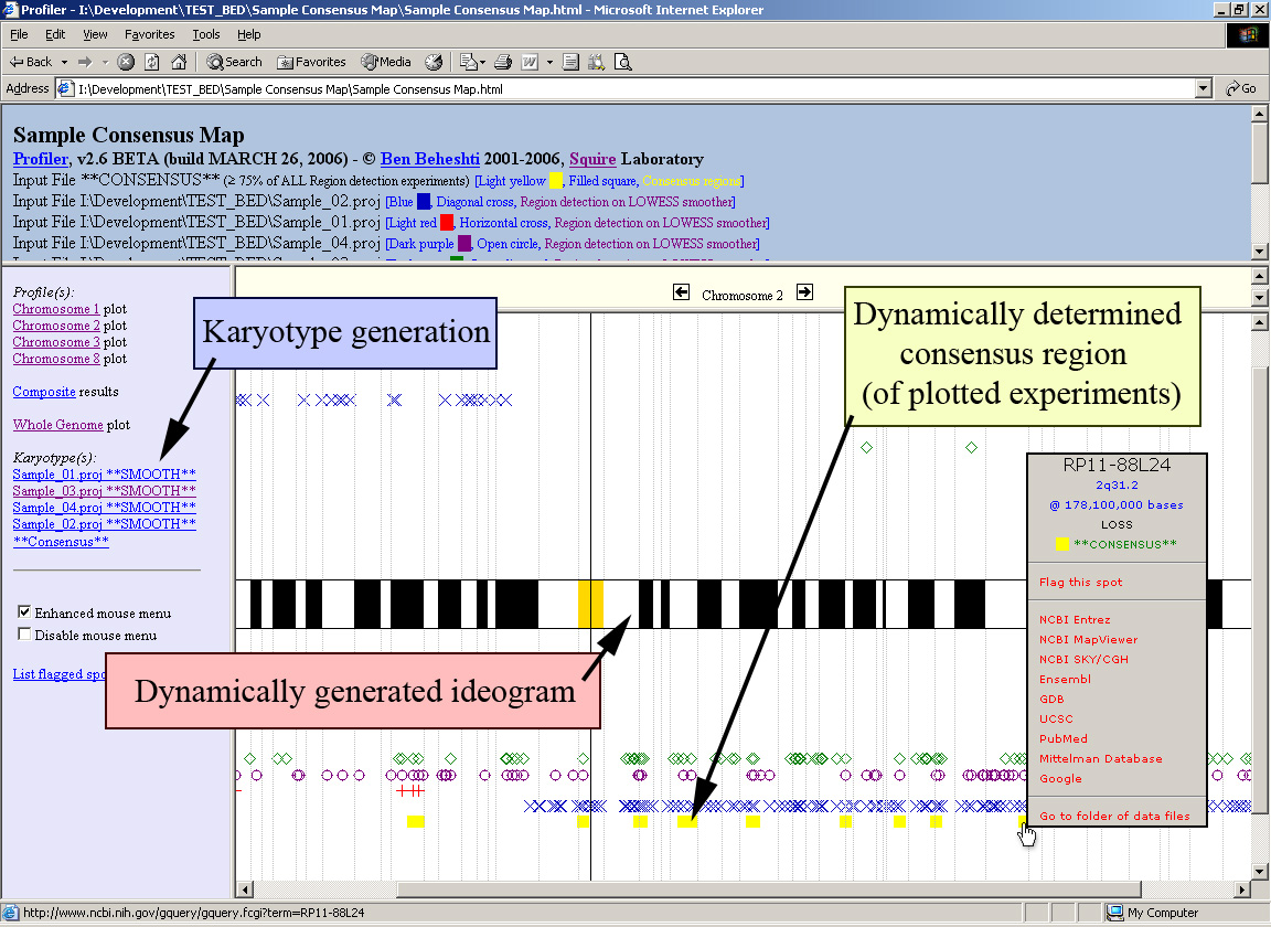
Profiler will generate the results images and launch your internet browser if HTML output is desired. Moving the mouse over data points in your internet browser will identify the clone, its cytoband, normalized intensity ratio, megabase position, and experiment name. Data points can be flagged into a "scratchpad", which can be used for keeping track of interesting clones for follow-up. It also provides a menu of convenient links to internet biological databases. An example of results generated by Profiler is given below, edited to include overlaid descriptions (click image to enlarge):
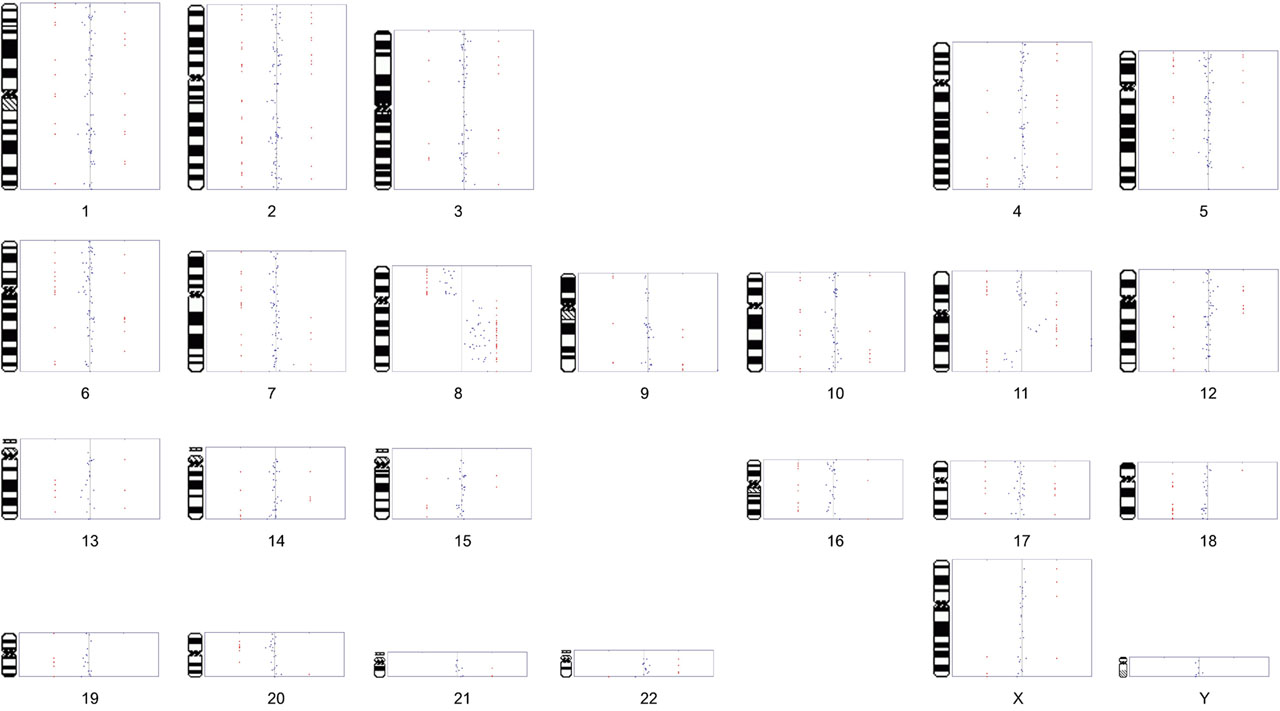
The software can also generate a composite karyotype image (results from all the chromosomes). As previously described, the red points indicate the spots that are gained/lost (here, at > 1 STD). Spots may be plotted as points (shown below) or connected with lines (click image to enlarge):
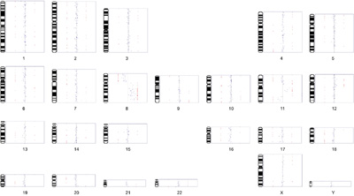
[Note: this is linked to a low-resolution image. The actual image is ~ 5 times larger and presentation-quality]
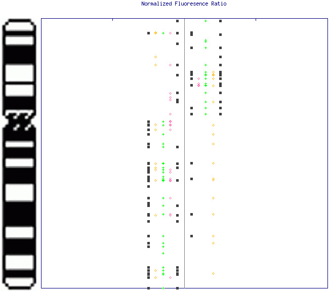
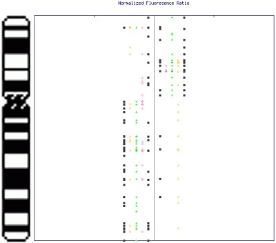
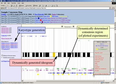
A consensus map of alterations can be quickly built by simply plotting all region detection data, to facilitate identification of consistent regions of change across interrogated samples. A composite image (similar to the image above) can be easily generated by the software, although the image shown below is a sample consensus map of changes on chromosome 6 created using five samples. Note the results may be viewed from within your internet browser to enable mouse-over of data points (as above) and link to internet biological databases (click image to enlarge):
Moreover, in addition to plotting a consensus map of changes, the software can determine the consensus regions of change amongst the plotted projects files (click image to enlarge):
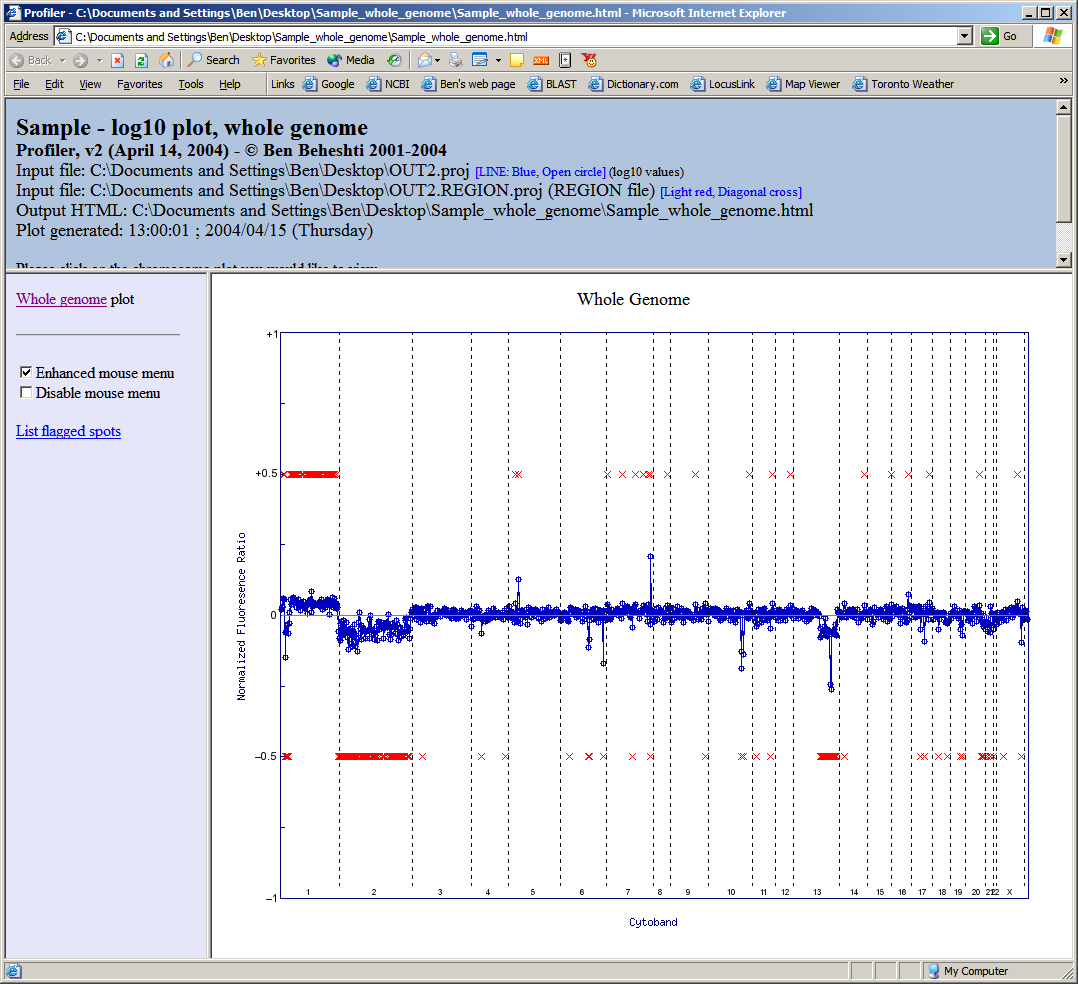
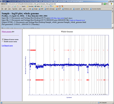
Lastly, one has the option of plotting the results across the whole genome in a single image. In the image below, results are plotted starting with chromosome 1 on the left and extend to chromosome X (and Y, if present) on the right. Note that region calling information can also be included to designate regions of copy number alteration. Also, if HTML output is selected, one can mouse-over the points for spot information and linking to internet biological databases (click image to enlarge):
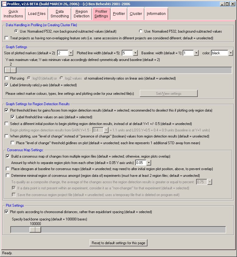
Note: The most commonly used settings are selected by default.
The images below show the profiler software user interface (click images to enlarge):


|
|
Citation
|

|
- Note: Users of the software suite can include the following citation:
- Chromosomal localization of DNA amplifications in neuroblastoma tumors using cDNA microarray comparative genomic hybridization.
- Ben Beheshti, Ilan Braude, Paula Marrano, Paul Thorner, Maria Zielenska, and Jeremy A. Squire.
- Neoplasia, 5(1):53-62, 2003.
- http://individual.utoronto.ca/beheshti/software/
- Access a PDF version of this paper.
- Results of this work are presented in the following posters: AACR, San Francisco 2002, and MSRD, 2003.

|
|
Contact
|
|
- Any questions, feedback, bug reports, ideas for new features, etc. are welcome. Please email Dr. Jeremy Squire (squirej@queensu.ca) or Dr. Ben Beheshti (ben.beheshti@utoronto.ca).
|
|