Sta107 Online Tutorial

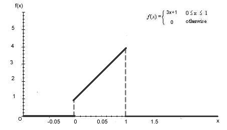
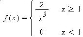
5.1 Probability Density Functions

We now consider random variables that can be measured on a continuous scale (time, distance, height, weight etc.)

Random variables measured on a continuous scales are uncountable, and is not possible to assign positive probability mass to all the outcomes. So we develop the idea of a probability density function.

Definition 5.1-1:

A random variable X is said to have a probability density function f(x) if for all x,

0 £ f(x)

and if for all values a and b

Random variables having such density functions are called continuous random variables.

Example 1:

Let random variable X have probability density function

To find P(0.01 £ X £ 0.07) we determine the area under the curve from 0.01 to 0.07. So P(0.01 £ X £ 0.07)=

What is P(0.03 £ X)?

(Round to 2 decimal places)

Solution

Example 2:

Refer to Example 5.1-2 on page 193 to help solve the follwing problem.

Let the random variable X have a probability density function

Find the value of c using the fact that the area under the curve must be 1.

Solution

Definition 5.1-2:

A random variable X is said to have a uniform distribution on the interval (c £ X £ d ) if

The random variable X will be referred to as a uniform [c,d] random variable.

If [a,b] is any subinterval of [c,d], then

Example 3:

Let the random variable X have the following uniform density function.

What is P(3£ X £ 4) ?

Using Definition 5.1-2, we know that a=3, b=4, c=3 and d=5.

So (b-a)/ (d-c) =(4-3)/(5-3)=1/2

What is P(3.2£ X £ 4.6) ?

(Round to 1 decimal place)

Solution

Example 4:

Let X have to following probability density function.

What is P(X>1)?

What is P(X>5)?

(Round to 2 decimal places)

Solution

Definition 5.1-3:

The cumulative distribution function of a continuous random variable X with probability density function f(x) is

The cumulative distribution function is just the area under the density function falling less than or equal to x.
When computing F(x) the actual limits of integration will depend on the domain over which f(x)>0.

Example 5:

Consider Example 1 again, where X had the following probability density function.

The cumulative distrubution can be found by integrating the function over its domain.

P(X £ 0.65)=F(0.65)=(3/2)(0.65)^2 +0.65=1.284

P(X>0.2)= 1-P(X £ 0.2) = 1-F(0.2)= 1- (3/2)(0.2)^2 -0.2 = 0.86

P( 0.1< X £ 0.42) =P( X £ 0.42) - P( X £ 0.1)

= F(0.42)-F(0.1)

= (3/2)(0.42)^2 +0.42 - [ (3/2)(0.1)^2 +0.1]

= 0.6846- 0.115

=0.5696

Round all answers to 2 decimal places

A: What is P(X£ 0.32)?

B: What is P(X>0.85)?

C: What is P( 0.4£ X £ 0.59)?

Solution

Useful Web Resources

Calculus Applied to Probability and Statistics by
Stefan Waner and Steven R. Costenoble

Cumulative Distribution Function- Wikipedia

Related Distributions

Solutions

Solution to Example 1

P(0.03 £ X)= P(0.03 £ X £ 1) because the upper bound on f(x) is 1. So P(0.03 £ X)=

Solution to Example 2

The area under the curve can be calculated as follows:

So c/18 must equal 1. c/18=1 implies that c=18.

x f(x)

0

0

0.5

1.5

1

0

The density function is

Solution to Example 3

Using definition 5.1-2, we know that a = 3.2, b= 4.6, c=3 and d=5.

So (b-a)/ (d-c) =(4.6-3.2)/(5-3)=0.7

Solution to Example 4

P(X>5)=P(X>=6), so

Solution to Example 5

A: P(X £ 0.32)=F(0.32)=(3/2)(0.32)^2 +0.32=0.47

B: P(X>0.85)= 1-P(X £ 0.85) = 1-F(0.85)= 1- (3/2)(0.85)^2 -0.85 = 1.23

C: P( 0.4£ X £ 0.59) =P( X £ 0.59) -P( X £ 0.4)

= F(0.59)-F(0.4)

= (3/2)(0.59)^2 +0.59 - [ (3/2)(0.4)^2 +0.4]

= 1.11215- 0.64

=0.47