The presence of nonlinearity in laws that govern the dynamics of a systems combined with nonequilibrium constraints can give rise to spatio-temporal self-organization phenomena. This diverse behavior is made possible from the multiple solutions which arise from the differential equations governing the kinetics found in such diverse fields as fluid dynamics, chemistry to more complex biological organisms[1].

At first glance the second law of thermodynamics, which is always pushing towards disorder, appears to counteract spontaneous formation of patterns. However, the emergence of order is made possible in dissipative structures, which are open systems that are able to export entropy into their environment and whose internal dynamics is dictated by irreversible processes far from equilibrium[2]. An understanding of nonlinear thermodynamic of far from equilibrium systems which forms the basis of pattern formation is a necessary first step and as such a qualitative and conceptual outline of nonequilibrium thermodynamics is provided here.

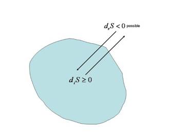
Figure 4 Open system

Evolution of an isolated system is generally described by the second law of thermodynamics, whereby the disorder or entropy S, in the system is increased until a maximum is reached at equilibrium. That is to say, in an isolated system we always have,

                                                (2.1)

Therefore, the spontaneous formation of patterns in an isolated system is not possible. Traditional thermodynamics, when describing a system that can exchange energy with the surroundings, does allow for ordered structures however, such as those found in crystals. The relative probability of these low energy structures, if we take E_n to represent a particular energy state of the system, is nonetheless given by the Boltzmann factor,

(2.2)

As can be seen from the above equation, low energy levels have an appreciable statistical preference only at low temperatures where effect of S is small. However, at higher temperatures, such as those encountered in living systems, the probability of existence for all states becomes more equal.

Thus in order to describe emergent patterns at room temperature and above, we have to look to open systems (see Figure 4), which are able to exchange energy and material with their surroundings. The change of entropy in such systems can be attributed to two factors:

1. Their internal entropy production , which is due to the irreversible processes inside the system and must necessary increase as dictated by the second law,

                                                           (2.3)

2. The entropy flux which is due to the exchange of energy and material.

In this way the total entropy change of the open systems is given by,

                                              (2.4)

Which can attain a state of lower total entropy in the presence of negative entropy flux,

                                                (2.5)

Furthermore, once such a lower entropy state or emergent patterns is formed, it can be maintained indefinitely provided,

                                              (2.6)

However for a system that is near equilibrium, the entropy flux term cannot be arbitrarily imposed, and thus an open system must meet a second requirement of far from equilibrium in order to exhibit emergent structure and patterns. Here we will demonstrate the restrictions on evolution of the system at and near thermodynamic equilibrium.

Much of the behavior of near equilibrium systems is dictated by properties and limitations of entropy production term, . Since we have to describe this term in a manner that is applicable to systems that can potentially exhibit inhomogeneity in time and space, it is most constructive to look at the change of entropy with respect to time and make use of a local description of entropy production σ, such that,

                                             (2.7)

and

                                                  (2.8)

Making use of mass balance equation, and local thermodynamic relations [2], the entropy production term can be described in terms of flows (J_k), associated with various irreversible processes k, taking place in the system  and the forces which influence them (X_k),

                                                  (2.9)

The flow term J_k describes factors such as rate of reaction per unit volume k and the diffusion flux ( ), while the forces that influence them X_k describe deviations from equilibrium that regulate the rate of reaction term and deviation of distribution of matter from equilibrium which affect diffusion.

At equilibrium the forces X_k as described above in terms of deviation vanish. Thus we can approximate that near equilibrium the forces remain weak and we can describe the flows J_k in power series expansion of X_k. This approximation leads to a near equilibrium relation of the form,

                                                 (2.10)

where  are phenomenological coefficients that define the internal structure of the medium. This linear relation combined with Onsanger’s reciprocity relation for the coefficients () restricts the production of entropy with respect to time and gives rise to

                                                           (2.11)

away from the equilibrium. And,

                                                           (2.12)

At equilibrium, where P is the total entropy production term which maintains the system in a non-equilibrium state. This essentially creates a stable node at equilibrium where any perturbation and order imposed on the system eventually dies out as the state approaches the stable equilibrium point. Furthermore as the equilibrium point is homogenous in space and time, any spontaneous emergent pattern must take place in a region where the linear relations between forces and flows are not applicable. Thus as we move away farther from equilibrium where the linear approximations break down, it is possible to have , where emergence of order is permitted.

In this way we have shown that it is possible for an open system to avoid a slow drift toward equilibrium and maintain its structure or even self organize into a lower entropy state by drawing negative entropy from the surroundings. It is important to note that oscillatory patterns which may arise in these systems are not going back and forth between thermodynamic equilibrium states but are all the while removed from equilibrium. These systems termed dissipative structures, can be considered the theoretical framework for most interesting phenomena found in nature, ranging from elementary functions of life to complex patterns of plants, animal skins, the atmosphere and most everything which does not decay to constant state.

As we’ll show later with experimental results from electrochemical systems, patterns in such nonlinear systems can evolve from initially stable homogenous structures given small perturbations. After the introduction of instability the nonlinear dynamics by which the components of the system interact, will define its pattern forming evolution. Furthermore the new patterns are entirely distinct from the initial instabilities and their linear functions introduced to the system. It is in fact this very ability of far from equilibrium nonlinear systems to map a set of potentially complex inputs to a generic pattern which we are proposing to exploit.

A prominent subclass of the nonlinear dynamical systems and one that is most relevant to the electrochemical system considered here is the reaction diffusion mechanism[3]. This is a very common description of macroscopic dynamics of complex systems. Here a full description would deal with infinite degrees of freedom that would describe each spatially distributed element as a function of time. For an electrochemical system this would mean a description of all ions and their interactions as function of time. While the sheer number of elements and the complexity of their dynamics is the very essence of computational power of the system, an analytical description requires certain simplifications and assumptions to reduce to the number of variables. It is important to emphasis here, that although analytical formulations and description of complex systems allow for better understanding of their internal dynamics and numerical solutions, they are by no means a complete portrait. A typical partial differential equation describing the evolution a spatially distributed, time variant system would require a large number of coupled equations, which may however be reduced to a finite number of variable equations of the of the form,

                     (2.13)

With representing each spatiotemporally active species and f_i the nonlinear reaction functions for all or a subset of variable described as c_j involved in the kinetics of c_i . The dynamics may involve a set of spatial derivatives  such as the Laplacian of temperature or concentration ΔT or Δc and D_j representing the constant of the spatial derivative. Furthermore, a set of spatiotemporally distributed external control parameters λ_x, like those described in the experimental section here, may be present in the system and have an effect on the kinetics.

1.         Coveney, P.V., Self-organization and complexity: a new age for theory, computation and experiment. Philosophical Transactions of the Royal Society of London Series a-Mathematical Physical and Engineering Sciences, 2003. 361(1807): p. 1057-1079.

2.         Nicolis, G. and I. Prigogine, Self-organization in nonequilibrium system : from dissipative structures to order through fluctuations. 1977, New York: Wiley. xii, 491 p.

3.         Epstein, I.R. and J.A. Pojman, An introduction to nonlinear chemical dynamics : oscillations, waves, patterns, and chaos. 1998, New York: Oxford University Press. xiv, 392 p.

Figure 1