Preface

This software is the result of my experiment to create a flexible numerical simulator. It solves a class of wave problems in acoustics. It consists the major components of a numerical software: a modeller in which scatterers can be constructed by stacking solids on top of each other, a gridder to generate the rectangular mesh, a solver that implements the numerical algorithm, some visualization and post processing capabilites.

Many efforts were spent on choosing the right architecture and the right tools. Object-oriented design patterns were used in the modeller. In the meantime, the numerical algorithm was implemented in a strictly procedural way. The XML format was chosen as the input file format as it was both human friendly and machine friendly. The H5 format was chosen due to the vast amount of data that could be potentially generated. I stayed with Matlab for the visualization and plotting needs.

There are many improvements that can be added to the software, such as handling inhomogeneous media, treating curve boundaries, parallelizing using OpenMP and MPI, optimizing the use of auxillary variables in the current implementation, generating animated plots, etc.. These will be considered when it comes with a research need.

In the meanwhile, if you want to comment on the software, want to see some features, or encounter any issue, feel free to inform me.

Thank you for the interest in this work.

G. Kevin Zhu

(g.kev.nosp@m.in.z.nosp@m.hu@ie.nosp@m.ee.o.nosp@m.rg)

Release History

If time permits, I am flexible to provide bug fixes and new features. Feel free to drop me a message. I expect to have a release every half a year.

Release 0.3 ( scheduled on 2014-01-01)
Release 0.2 ( on 2013-07-01)
- Add the executable "ac2d", which reads a script file in the XML format and stores the data in a file in the H5 format.
- Update the validation examples, which demonstrate the use of "ac2d" and the CPP interface.
- Add the support of the uniaxial perfectly matched layers (U-PML) in "ac2d" so that the memory consumption is reduced.
- Add the option in "ac2d" to estimate the optimal values of the PML parameters based on the settings in the input file.
Release 0.1 (on 2013-03-23) - Initial release.

Table of Contents

Introduction

Acoustic FDTD Solver (AC2D) is a software to simulate acoustic wave propagation in lossy media in two dimensions. It uses the finite-difference time-domain (FDTD) method to solve the wave equation. It has the following features

Simulate the 2-D acoustic wave propagation in lossy media. The particle velocity is in the plane of propagation, i.e. perpendicular polarization.
Implement a hard point source and a hard plane wave source at an oblique angle.
Support the pressure-release boundary condition, the rigid boundary condition, and the periodic boundary condition. The infinite boundary condition is realized through the complex frequency shifted perfectly matched layers (CFS-PML) [Gedney2005].
Record the pressure field at a point and along a line.

The software provides an executable called "ac2d", which reads a script file in the XML format as the input argument and stores the field values in an output file in the H5 format. The software also provides an easy-to-use C++ interface for experienced developers to explore its functionality.

The software can be used to solve the following practical problems

Solve for the wave scattered by acoustic objects due to a plane wave or an isotropically radiated wave.
Find the reflection coefficient and the transmission coefficient of stratified media.
Can be configured to run sub-band FDTD simulations to simulation wave propagation in linearly dispersive media [Zhao2006].

The software has been test and validated on Linux and Mac OS X. It depends on the following external software

RapidXML to parse the input script file.
HDF5 library to store data in the output file.
Boost program_options library to parse the command line arguments.
Matlab to generate the figures in the validation examples.
Doxygen to generate this documentation.

The software is placed under the open BSD license.

Linear Acoustic Theory

In linear acoustic theory [Kinsler2000], the two field quantities, the acoustic pressure denoted by $p$ and the particle velocity denoted by $\vec{u}$ , are related by the continuity equation, which is given by

$\frac{\partial p}{\partial t} = -K\nabla\cdot\vec{u} - \xi K p$

and the simple force equation, which is given by

$\frac{\partial \vec{u}}{\partial t} = -\frac{1}{\rho}\nabla p -\frac{\xi^\ast}{\rho} \vec{u} \label{E:force}\ \$

where

denotes the bulk modulus.
$\rho$ denotes the density.
$\xi$ denotes the loss associated with the acoustic pressure.
$\xi^{\ast}$ denotes the loss associated with the particle velocity.

Due to the large medium intrinsic impedance ( $\eta_0=\sqrt{\rho_0 K_0}\sim 10^6$ ), we introduce the quantities normalized with respect to the impedance $\widetilde{\vec{u}}=\eta_0\vec{u}$ , $\widetilde{\rho}=\rho/\eta_0$ , and $\widetilde{K}= K/\eta_0$ . The continuity equation and the simple force equation with the normalized quantities become

$\frac{\partial p}{\partial t} = -\widetilde{K}\nabla\cdot\widetilde{\vec{u}} - \xi K p$

$\frac{\partial \widetilde{\vec{u}}}{\partial t} = -\frac{1}{\widetilde{\rho}}\nabla p - \frac{\xi^\ast}{\rho} \widetilde{\vec{u}}$

Converting the time-domain equations to the frequency domain (using the $e^{j\omega t}$ time-harmonic factor) gives

$j\omega {P} = -\widetilde{K}\nabla\cdot\widetilde{\vec{U}} - \xi K P \label{E:ac_freq_cont}$

$j\omega \widetilde{\vec{U}} = -\frac{1}{\widetilde{\rho}}\nabla P -\frac{\xi^\ast}{\rho} \widetilde{\vec{U}} \label{E:ac_freq_force}\\$

where the upper case letters denote the frequency-domain quantities.

The complex stretch factor in the CFS-PML modifies the spatial derivatives, which is given by

$\frac{\partial}{\partial s} \to \left(\kappa_s + \frac{\xi_s}{\alpha_s+j\omega}\right)^{-1} \frac{\partial}{\partial s}$

where $\alpha_s$ , $\kappa_s$ and $\xi_s$ are the parameters in the CFS-PML. The subscript $s$ can be $x$ , $y$ , or $z$ . The continuity equation, under this stretch-coordinate transformation, becomes

$j\omega P = -\widetilde{K}\sum_{s\in\{x,y,z\}} \frac{1}{\kappa_s}\left[1 - \frac{\xi_s}{(\alpha_s+j\omega)\kappa_s+\xi_s}\right]\frac{\partial \widetilde{U}_s}{\partial s} - \xi K P$

The simple force equation, under this transformation, becomes

$j\omega\widetilde{U}_s = -\frac{1}{\widetilde{\rho}\kappa_s} \left[ 1 - \frac{\xi_s}{(\alpha_s+j\omega)\kappa_s + \xi_s}\right]\frac{\partial P}{\partial s} - \frac{\xi^\ast}{\widetilde{\rho}} \widetilde{U}_s$

One popular implementation of the CFS-PML is known as the convolutional PML. Here we use the other implementation, known as the auxiliary differential equation method. Let us define an auxiliary variable $B_s$ (note that $B_s$ is spatially and temporally co-located with $P$ ), which is

$B_s = - \frac{\xi_s}{(\alpha_s+j\omega)\kappa_s + \xi_s}\frac{\partial \widetilde{U}_s}{\partial s}$

and another auxiliary variable $A_s$ (note that $A_s$ is spatially and temporally co-located with $\widetilde{U}_s$ ), which is

$A_s = - \frac{\xi_s}{(\alpha_s+j\omega)\kappa_s + \xi_s}\frac{\partial P}{\partial s}$

Using the newly introduced variables, the transformed continuity equation is given by

$j\omega P = -\widetilde{K} \sum_{s\in\{x,y,z\}}\frac{1}{\kappa_s} \left(\frac{\partial \widetilde{U}_s}{\partial s}+B_s\right)-\xi K P$

The transformed simple force equation is given by

$j\omega\widetilde{U}_s = -\frac{1}{\widetilde{\rho}\kappa_s} \left( \frac{\partial P}{\partial s} + A_s\right) - \frac{\xi^\ast}{\widetilde{\rho}} \widetilde{U}_s$

The auxiliary differential equations that consist of the parameters of the CFS-PML are given by

$j\omega B_s = -\frac{\xi_s}{\kappa_s}\frac{\partial \widetilde{U}_s}{\partial s} - \left(\alpha_s+\frac{\xi_s}{\kappa_s} \right)B_s \hspace{2ex}.$

$j\omega A_s = -\frac{\xi_s}{\kappa_s}\frac{\partial P}{\partial s} - \left(\alpha_s+\frac{\xi_s}{\kappa_s} \right)A_s \label{E:A_update}$

The corresponding time-domain equations are given by

$\frac{\partial}{\partial t} b_s = -\frac{\xi_s}{\kappa_s} \frac{\partial}{\partial s} \widetilde{u}_s - (\alpha_s + \frac{\xi_s}{\kappa_s}) b_s$

$\frac{\partial}{\partial t} p = -\widetilde{K}\sum_{s\in\{x,y,z\}} \frac{1}{\kappa_s}(\frac{\partial}{\partial s}\widetilde{u}_s + b_s)-\xi K p$

$\frac{\partial}{\partial t} a_s = -\frac{\xi_s}{\kappa_s} \frac{\partial}{\partial s} p - (\alpha_s + \frac{\xi_s}{\kappa_s}) a_s$

$\frac{\partial}{\partial t} \widetilde{u}_s = -\frac{1}{\widetilde{\rho}\kappa_s}(\frac{\partial}{\partial s} p + a_s)-\frac{\xi^\ast}{\widetilde{\rho}} \widetilde{u}_s$

where the lower case letters denote the time-domain quantities.

Finite-Difference Time-Domain Method

Let $\Delta x$ , $\Delta y$ and $\Delta z$ denote the spatial increments along the $x$ , $y$ and $z$ directions. Let $\Delta t$ denote the temporal increment. The acoustic pressure is located at the integer multiple of the spatial increments and the temporal increment. For instance, $p|_{i,j,k}^n$ denotes the acoustic pressure at the location $(i\Delta x, j\Delta y, k\Delta z)$ and at the time $n\Delta~t$ . The normalized particle velocity is located at the half-integer multiple of the spatial increments and the temporal increment. For instance, $\widetilde{u}_x|_{i+\frac{1}{2},j,k}^{n+\frac{1}{2}}$ denotes the normalized particle velocity in the $x$ direction at the location $((i+\frac{1}{2})\Delta x, j\Delta y, k\Delta z)$ and at the time $(n+\frac{1}{2})\Delta~t$ . The adopted Yee cell in the y-z plane is shown below.

Acoustic Yee cell

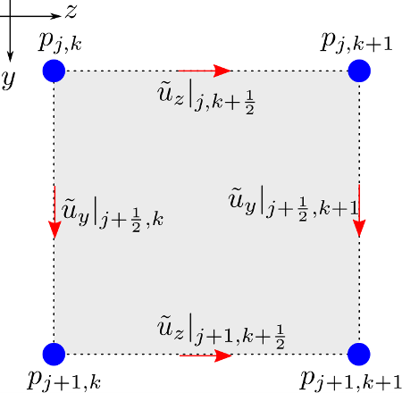
The central-difference approximation of the time-domain equations are given by

$b_x|_{i,j,k}^n = \frac{2-(\alpha_x+\xi_x/\kappa_x)\Delta t}{2+(\alpha_x+\xi_x/\kappa_x)\Delta t}{} b_x|_{i,j,k}^{n-1} - \frac{2(\Delta t \xi_x)/(\Delta x \kappa_x)}{2+(\alpha_x+\xi_x/\kappa_x)\Delta t}{}\left(\widetilde{u}_x|_{i+\frac{1}{2},j,k}^{n-\frac{1}{2}} - \widetilde{u}_x|_{i-\frac{1}{2},j,k}^{n-\frac{1}{2}} \right)$

$b_y|_{i,j,k}^n = \frac{2-(\alpha_y+\xi_y/\kappa_y)\Delta t}{2+(\alpha_y+\xi_y/\kappa_y)\Delta t}{} b_y|_{i,j,k}^{n-1} - \frac{2(\Delta t \xi_y)/(\Delta y \kappa_y)}{2+(\alpha_y+\xi_y/\kappa_y)\Delta t}{}\left(\widetilde{u}_y|_{i,j+\frac{1}{2},k}^{n-\frac{1}{2}} - \widetilde{u}_y|_{i,j-\frac{1}{2},k}^{n-\frac{1}{2}} \right)$

$b_z|_{i,j,k}^n = \frac{2-(\alpha_z+\xi_z/\kappa_z)\Delta t}{2+(\alpha_z+\xi_z/\kappa_z)\Delta t}{} b_z|_{i,j,k}^{n-1} - \frac{2(\Delta t \xi_z)/(\Delta z \kappa_z)}{2+(\alpha_z+\xi_z/\kappa_z)\Delta t}{}\left(\widetilde{u}_z|_{i,j,k+\frac{1}{2}}^{n-\frac{1}{2}} - \widetilde{u}_z|_{i,j,k-\frac{1}{2}}^{n-\frac{1}{2}} \right)$

$p|_{i,j,k}^n = \frac{2-\Delta t \xi K}{2+\Delta t \xi K}p|_{i,j,k}^{n-1} - \left( \frac{\Delta t \tilde{K}/\kappa_x}{2+\Delta t \xi K} \left(b_x|_{i,j,k}^n + b_x|_{i,j,k}^{n-1}\right) + \frac{\Delta t \tilde{K}/\kappa_y}{2+\Delta t \xi K} \left(b_y|_{i,j,k}^n + b_y|_{i,j,k}^{n-1}\right) + \frac{\Delta t \tilde{K}/\kappa_z}{2+\Delta t \xi K} \left(b_z|_{i,j,k}^n + b_z|_{i,j,k}^{n-1}\right) \right)$

$- \left( \frac{(2\Delta t \widetilde{K})/(\Delta x \kappa_x)}{2+\Delta t \xi K}\left(u_x|^{n-\frac{1}{2}}_{i+\frac{1}{2},j,k} - u_x|^{n-\frac{1}{2}}_{i-\frac{1}{2},j,k} \right) + \frac{(2\Delta t \widetilde{K})/(\Delta y \kappa_y)}{2+\Delta t \xi K}\left(u_y|^{n-\frac{1}{2}}_{i,j+\frac{1}{2},k} - u_y|^{n-\frac{1}{2}}_{i,j-\frac{1}{2},k} \right) + \frac{(2\Delta t \widetilde{K})/(\Delta z \kappa_z)}{2+\Delta t \xi K}\left(u_z|^{n-\frac{1}{2}}_{i,j,k+\frac{1}{2}} - u_z|^{n-\frac{1}{2}}_{i,j,k-\frac{1}{2}} \right) \right)$

$a_x|_{i+\frac{1}{2},j,k}^{n+\frac{1}{2}} = \frac{2-(\alpha_x+\xi_x/\kappa_x)\Delta t}{2+(\alpha_x+\xi_x/\kappa_x)\Delta t}{} a_x|_{i+\frac{1}{2},j,k}^{n-\frac{1}{2}} - \frac{2(\Delta t \xi_x)/(\Delta x \kappa_x)}{2+(\alpha_x+\xi_x/\kappa_x)\Delta t}{}\left(p|_{i+1,j,k}^{n} - p|_{i,j,k}^{n} \right)$

$a_y|_{i,j+\frac{1}{2},k}^{n+\frac{1}{2}} = \frac{2-(\alpha_y+\xi_y/\kappa_y)\Delta t}{2+(\alpha_y+\xi_y/\kappa_y)\Delta t}{} a_y|_{i,j+\frac{1}{2},k}^{n-\frac{1}{2}} - \frac{2(\Delta t \xi_y)/(\Delta y \kappa_y)}{2+(\alpha_y+\xi_y/\kappa_y)\Delta t}{}\left(p|_{i,j+1,k}^{n} - p|_{i,j,k}^{n} \right)$

$a_z|_{i,j,k+\frac{1}{2}}^{n+\frac{1}{2}} = \frac{2-(\alpha_z+\xi_z/\kappa_z)\Delta t}{2+(\alpha_z+\xi_z/\kappa_z)\Delta t}{} a_z|_{i,j,k+\frac{1}{2}}^{n-\frac{1}{2}} - \frac{2(\Delta t \xi_z)/(\Delta z \kappa_z)}{2+(\alpha_z+\xi_z/\kappa_z)\Delta t}{}\left(p|_{i,j,k+1}^{n} - p|_{i,j,k}^{n} \right)$

$\widetilde{u}_x|^{n+\frac{1}{2}}_{i+\frac{1}{2},j,k} = \frac{2-\Delta t\xi^\ast/\widetilde{\rho}}{2+\Delta t\xi^\ast/\widetilde{\rho}}\widetilde{u}_x|^{n-\frac{1}{2}}_{i+\frac{1}{2},j,k} -\frac{ \Delta t/(\widetilde{\rho}\kappa_x)}{2+\Delta t\xi^\ast/\widetilde{\rho}}\left(a_x|^{n+\frac{1}{2}}_{i+\frac{1}{2},j,k} + a_x|^{n-\frac{1}{2}}_{i+\frac{1}{2},j,k}\right) -\frac{2\Delta t/(\widetilde{\rho}\kappa_x \Delta x)}{2+\Delta t \xi^\ast/\widetilde{\rho}}\left(p|^n_{i+1,j,k}-p|^n_{i,j,k}\right)$

$\widetilde{u}_y|^{n+\frac{1}{2}}_{i,j+\frac{1}{2},k} = \frac{2-\Delta t\xi^\ast/\widetilde{\rho}}{2+\Delta t\xi^\ast/\widetilde{\rho}}\widetilde{u}_y|^{n-\frac{1}{2}}_{i,j+\frac{1}{2},k} -\frac{ \Delta t/(\widetilde{\rho}\kappa_y)}{2+\Delta t\xi^\ast/\widetilde{\rho}}\left(a_y|^{n+\frac{1}{2}}_{i,j+\frac{1}{2},k} + a_y|^{n-\frac{1}{2}}_{i,j+\frac{1}{2},k}\right) -\frac{2\Delta t/(\widetilde{\rho}\kappa_y \Delta y)}{2+\Delta t \xi^\ast/\widetilde{\rho}}\left(p|^n_{i,j+1,k}-p|^n_{i,j,k}\right)$

$\widetilde{u}_z|^{n+\frac{1}{2}}_{i,j,k+\frac{1}{2}} = \frac{2-\Delta t\xi^\ast/\widetilde{\rho}}{2+\Delta t\xi^\ast/\widetilde{\rho}}\widetilde{u}_z|^{n-\frac{1}{2}}_{i,j,k+\frac{1}{2}} -\frac{ \Delta t/(\widetilde{\rho}\kappa_z)}{2+\Delta t\xi^\ast/\widetilde{\rho}}\left(a_z|^{n+\frac{1}{2}}_{i,j,k+\frac{1}{2}} + a_z|^{n-\frac{1}{2}}_{i,j,k+\frac{1}{2}}\right) -\frac{2\Delta t/(\widetilde{\rho}\kappa_z \Delta z)}{2+\Delta t \xi^\ast/\widetilde{\rho}}\left(p|^n_{i,j,k+1}-p|^n_{i,j,k}\right)$

The software implements the update equations in the following order: $b_s \to p \to a_s \to \tilde{u}_s \to b_s$ . The implementation is in ACFDTD22::execute().

Download and Installation

Preparation on Ubuntu Linux

Enter the following command in a terminal to install the needed libraries

 $ sudo apt-get install libboost-program-options  libhdf5-serial-dev

Preparation on Mac OS X

The following steps are needed before compiling the software on Mac OS X

Install XCode, the integrated development environment from the App Store or from https://developer.apple.com/xcode/, free from Apple.
Inside XCode, go to XCode->Preferences->Downloads->Command Line Tools. This installs the development tools on the operating system, such as GCC/G++, make, svn, etc.
Install MacPorts, a system for developing open-source software on Mac OS X. The installer of MacPorts can be obtained from http://www.macports.org/install.php.
Open a terminal, and enter the following command to install the HDF5 library
```
 $ sudo port install hdf5-18
```

The latest Boost source code can be obtained from http://www.boost.org/users/download/. Download the file "boost_1_51_0.tar.gz", and enter the following commands in a terminal to build Boost.

 $ gunzip boost_1_51_0.tar.gz
 $ tar xvf boost_1_51_0.tar
 $ cd boost_1_51_0/
 $ bash ./bootstrap      # This collects the information on the operating system.
 $ sudo ./bjam install   # This may take around 20 minutes depending on the speed of the computer.

Preparation on Windows

Although this code has not been tested on Windows, it is expected to run in Cygwin, the Linux-like environment for Windows. The HDF5 library, Boost library, and Doxygen are all available in the Package Selection Window in the Cygwin installer.

Obtaining the source code

The stable release of the source code can be obtained from http://sourceforge.net/projects/ac2d/files/?source=navbar. To extract the source code from this file, enter the following commands in a terminal.

 $ unzip AC2D-<release number>.zip

If you have difficulty to download the file, you can access the stable release of the source code in the SVN repository hosted by SourceForge. You can see the available stable releases by entering the following command in a terminal.

 $ svn ls svn://svn.code.sf.net/p/ac2d/code

You can checkout the stable release by entering the following command.

 $ svn checkout svn://svn.code.sf.net/p/ac2d/code/tags/<release number> ac2d

If you want to follow the latest development of the software, you can access the code in the SVN trunk by entering the following command.

 $ svn checkout svn://svn.code.sf.net/p/ac2d/code/trunk ac2d

Compilation and Installation

To install the software, enter the following commands in a terminal. This generates the executable "ac2d" and places it under ac2d/bin. It also generates the library "libac2d.a" and places it under ac2d/lib.

 $ cd ac2d
 $ make
 $ make install

Using "ac2d"

The help message of "ac2d" is listed below.

NAME
ac2d - Software to simulate acoustic wave propagation in lossy media in two dimensions.

SYNOPSIS
ac2d [-m] [-pml --alpha_max=sweep --xi_ratio=sweep] <file_name>.ac2d

DESCRIPTION
The executable reads the input script file and invokes the FDTD
simulation. The output is stored in the file <file_name>.h5.

OPTIONS
--input-file=<file_name>.ac2d
--pml Estimate the optimal values of the CFS-PML parameter
\alpha_max and \xi_ratio. This takes the grid setting
and the excitation setting (must be a GaussianModulatedSinusoid)
from the input script file. It runs one simulation over a large
domain and runs multiple simulations for all the combinations of
the possible values of \alpha_max and \xi_ratio on a small
domain. It identifies the optimal values, which yield the
smallest relative error as defined in (7.135) in [Taflove2005].
--alpha_max=lb:step:ub Specify the range between "lb" and "ub", in which the optimal value
of \alpha_max, the shifting term, is estimated at the increment of
"step". The sweep range is default to (0:0.1:1.0).
--xi_ratio=lb:step:ub Specify the range between "lb" and "ub", in which the optimal value
of \xi_ratio, the ratio with respect to the optimal loss defined
in (7.62) in [Taflove2005], is estimated at the increment of "step".
The sweep range is default to (0:0.1:1.0).
--mem Use U-PML instead of CFS-PML. It sets \kappa=1.0 and \alpha=0.0 in
the PML region. This reduces the memory consumption.
--help Display this help message.
--version Display the version information.

AUTHOR
Written by Guangran Kevin Zhu.

REPORTING BUGS
Report bugs to g.kevin.zhu@ieee.org

Using the C++ Interface

See the files placed in ac2d/validation/cpp_interface.

Numerical Validation

There are three validation examples provided in this software and they are placed under ac2d/validation. The first two examples demonstrate the use of "ac2d" and the CPP interface. The third example uses the CPP interface only.

Performance of the CFS-PML

This example demonstrates the efficiency of the CFS-PML to absorb the outgoing waves. Consider a pressure pulse injected at the centre of the acoustic domain as shown in the figure below. The background has a density of 1 kg/m^3 and an acoustic speed of 1 m/s. A pressure pulse is imposed at Location O, the centre of the domain. The domain is terminated by the CFS-PML in the y-direction and the z-direction. The cell size is 0.1 m in both directions, which corresponds to 10 points per wavelength at the centre frequency. Location A is 5 cells away from the PML boundary, and Location B is 5 cells away from the neighbouring two boundaries. The relative CFL number is 0.99, which translates to a temporal increment of 7.0004e-02 s.

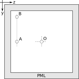
Two-dimensional simulation domain to study the absorption capability of the CFS-PML.

Three simulations are executed. One simulation is run with 5 PML layers on each boundary. The simulation domain has 130x130 cells. Another simulation is run with 10 PML layers on each boundary. The simulation domain has 140x140 cells. The third simulation has no PML layers. The simulation domain has 1344x1344 cells.

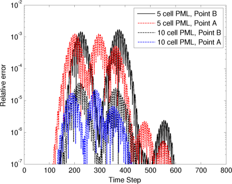
The pressure fields at Location A and B are recorded in the three simulations. The difference in the pressure fields between the simulations with the PML layers and the simulation without any PML layer is a measure of the ability of the CFS-PML to absorb outgoing waves. This leads to the definition of a relative error given by (7.135)[Taflove2005]

$Relative\hspace{1ex}error|_{j,k}^n=\frac{|p|_{j,k}^n-p_{ref}|_{j,k}^n|}{\max[p_{ref}|_{j,k}^n]}$

The relative errors are shown in the figure below.

Relative error at points A and B in the computation domain

To run this validation example using "ac2d", enter the following commands in a terminal.

 $ cd ac2d/validation/xml_interface 
 $ bash pml_benchmark.sh

To run this validation example through the CPP interface, enter the following commands in a terminal.

 $ cd ac2d/validation/cpp_interface 
 $ make pml_benchmark
 $ bash pml_benchmark.sh

Inside Matlab, enter the following commands to generate the figures.

 >> cd ac2d/validation
 >> plotCFLPMLBenchmark('xml_interface');
 >> plotCFLPMLBenchmark('cpp_interface');

The two figure should be identical.

Normal Incident Plane Wave Scattered by a Cylinder

Consider a plane wave in a homogeneous medium normally incident on a cylinder as shown below. The homogeneous medium is characterized by an intrinsic impedance $\eta_0$ . The cylinder is characterized by an intrinsic impedance $\eta_1$ and a radius $a$ .

Plane wave scattered by a cylinder.

The incident field and the scattered field at the location $(r,\phi)$ are given by

$p_{inc}(r, \phi) = \sum^{+\infty}_{n=-\infty} j^{-n} J_n(k_0 r) e^{jn\phi}$

$p_{scat}(r,\phi) = \sum^{+\infty}_{n=-\infty} a_n H_n^{(2)} (k_0 r) e^{jn\phi}$

where

$a_n = j^{-n} \frac{\eta_0 J_n(k_0 a) J_n{'}(k_1a) - \eta_0 J_n(k_1 a) J_n{'}(k_0 a)}{\eta_0 H^{(2)}{'}(k_0 a) J_n(k_1 a) - \eta_0 H_n^{(2)}(k_0 a) J_n{'}(k_1 a)}$

The analytical expression of the field scattered by a dielectric cylinder can be found in [Balanis1989].

Consider the numerical example shown in the following figure. The background has a density of 1 kg/m^3 and an acoustic speed of 1 m/s. The cylinder has a density of 1 kg/m^3 and an acoustic speed of 0.8 m/s. It has a radius of 1 m and is centered at (9, 20). The incident pulse is a Gaussian-modulated sinusoid centered at 1 Hz. The standard deviation of the envelope is 0.5 s. The simulation domain is terminated by a 10-layer PML in the y-direction, and by the periodic boundaries in the z-direction. The domain has 480x1200 cells. The cell size is 0.05 m in both directions, which corresponds to 30 points per wavelength at the centre frequency. The relative CFL number is 0.99, which translates to a temporal increment of 2.3334e-02 s.

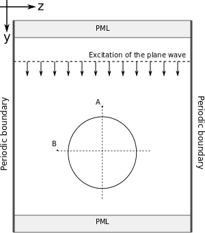
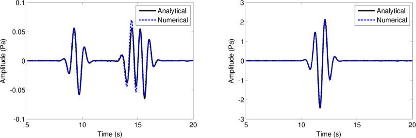
Two dimensional simulation domain which models a plane wave scattered by an acoustic cylinder.

Two FDTD simulations, one with the cylinder and one without the cylinder, are executed. The difference between the fields of the two simulations gives the scattered fields at Location A and B, which are 2 m away from the centre of the cylinder. Some Matlab code is borrowed from Cylinder Scattering [CS2011], which calculates the scattered field using the analytical expression. The comparisons between the analytic solutions and the numerical solutions of the scattered fields at Location A and B are shown below. The differences between the curves are due to numerical dispersion in the FDTD method.

Scattered acoustic pressures at Location A and B.

To run this example using "ac2d", enter the following commands in a terminal.

 $ cd ac2d/validation/xml_interface
 $ bash plane_wave_cylinder.sh

To run this example through the CPP interface, enter the following commands in a terminal.

 $ cd ac2d/validation/cpp_interface
 $ make plane_wave_cylinder
 $ bash plane_wave_cylinder.sh

Inside Matlab, enter the following commands to generate the figures.

 >> cd ac2d/validation
 >> generateCylinderScatteredField
 >> plotCylinderScatteredField('xml_interface');
 >> plotCylinderScatteredField('cpp_interface');

The two figures should be identical.

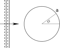
Obliquely Incident Plane Wave Reflected by a Half Space

This example demonstrates the obliquely incident plane wave reflected by a half space. Consider a plane wave in a homogeneous medium characterized by an intrinsic impedance $\eta_0$ , obliquely incident at an angle $\theta_i$ on a half space characterized by an intrinsic impedance $\eta_1$ . The plane wave is reflected at an angle $\theta_i$ and refracted at an angle $\theta_t$ as shown below.

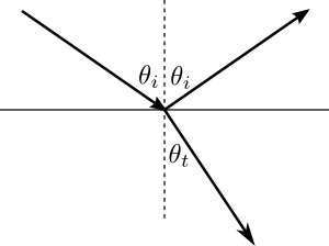
Plane wave obliquely incident upon a half-space

The particle velocities are in the plane of incidence. This corresponds to the perpendicular polarization in electromagnetics. The reflection coefficient, denoted by $\Gamma$ , is given by

$\Gamma = \frac{\eta_1\cos(\theta_i)-\eta_0\cos(\theta_t)}{\eta_1\cos(\theta_i)+\eta_0\cos(\theta_t)}$

and the transmission coefficient, denoted by $\tau$ , is given by

$\tau = \frac{2\eta_1\cos(\theta_i)}{\eta_1\cos(\theta_i)+\eta_0\cos(\theta_t)}$

The angle at which the reflection coefficient is 0 is known as the intromission angle. This angle is the same as the Brewster angle of no reflection in electromagnetics. The Brewster angle for the perpendicular polarization in electromagnetics is not easily observed, since naturally occurring materials usually have very similar permeabilities. In acoustics, if the density and the velocity of the background and the half space satisfy the following relationship [DAguanno2012]

$\frac{(\rho_1/\rho_0)^2-(c_0/c_1)^2}{(\rho_1/\rho_0)^2-1} > 0$

then the acoustic intromission angle is given by

$\theta_{intromission}= \arcsin\left( \sqrt{\frac{(\rho_1/\rho_0)^2-(c_0/c_1)^2}{(\rho_1/\rho_0)^2-1} }\right)$

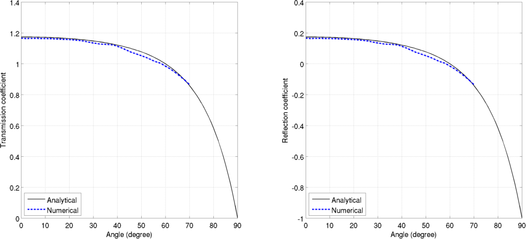
Consider the numerical example shown in the following figure. The background has a density of 1 kg/m^3 and an acoustic speed of 1 m/s. The medium has a density of 1.75 kg/m^3 and an acoustic speed of 0.81228 m/s. A time-harmonic plane wave with a unity amplitude at 1 Hz incidents at an angle, and the perfectly matched layer are used at the four boundaries to terminate the simulation domain. There are 30 points allocated per wavelength. The CFL number is 0.99, which translates to the temporal increment of 3.500e-02 s.

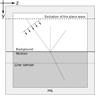
Two-dimensional simulation domain which models a plane wave reflected by an acoustic medium.

At each incident angle, two FDTD simulations, one without the acoustic half space and one with the acoustic half space, are executed. The difference in the field values recorded along the line sensor in the two simulations is the refracted wave. The reflection coefficient is the magnitude ratio between the reflected wave and the incident wave. The transmission coefficient is the magnitude ratio between the refracted wave and the incident wave. These angle-dependent coefficients are shown below. It is observed that, when the incident angle is 60 degrees, the reflection coefficient is 0.

Transmission and reflection coefficients.

To run this validation example, enter the following commands in a terminal.

 $ cd ac2d/validation/cpp_interface
 $ make plane_wave_reflection
 $ bash plane_wave_reflection.sh

Inside Matlab, enter the following commands to generate the figures.

 >> cd ac2d/valication
 >> plotHalfspaceTransmissionCoefficient('cpp_interface');

Currently, this example is not supported by "ac2d".

Additional Topics

Generating this Document

This software document in the HTML format can be generated by entering the following commands in a terminal.

 $ cd ac2d
 $ make doc
 $ firefox doc/html/index.html

References

[Balanis1989] C. A. Balanis, Advanced Engineering Electromagnetics. New York, NY: John Wiley & Sons, Inc., 1989.

[CS2011] G. K. Zhu. Cylinder scattering. Online. [Online]. Available: http://www.mathworks.com/matlabcentral/fileexchange/30162-cylinder-scattering

[DAguanno2012] G. D'Aguanno, K. Q. Le, R. Trimm, A. Alù, N. Mattiucci, A. D. Mathias, N. Aközbek, and M. J. Bloemer, "Broadband metamaterial for nonresonant matching of acoustic waves," Scientific Reports 2, no. 340, pp. 1–5, 2012.

[Gedney2005] S. D. Gedney, "Perfectly matched layer absorbing boundary conditions," in Computational Electrodynamics: the Finite-Difference Time-Domain Method, A. Taflove and S. C. Hagness, Eds., 3rd ed. Boston, MA: Artech House, 2005, ch. 9.

[Kinsler200] L. E. Kinsler, A. R. Frey, A. B. Coppens, and J. V. Sanders, Fundamentals of Acoustics. New York, NY: John Wiley & Sons, Inc., 2000.

[Zhao2006] Y. Zhao, Y. Hao, A. Alomainy, and C. Parini, "UWB on-body radio channel modeling using ray theory and subband FDTD method," IEEE Trans. Microw. Theory Tech., vol. 54, no. 4, pp. 1827–1835, Apr. 2006.