|
Example 1| Example 2 | Exercise 2.7-6 | Theorem 2.7-4 |Useful Web Resources| Solutions
Theorem 2.7-1:
Let X and Y have joint probability mass function p(x,y). Let W=Q(X,Y). Then,
Example 1:
Let X and Y have joint probability mass function.
x |
y |
p(x,y) |
0 |
1 |
2 |
| 1 |
0.15 |
0.10 |
0.25 |
| 2 |
0.35 |
0.10 |
0.05 |
Let W=(X^2)Y
E(W)= (1)^2(1)(0.10) + (2^2)(1)(0.25) +
(1^2)(2)(0.10) + (2^2)(2)(0.05) =
Let W=X(Y^2). What is E(W)?
Solution 
Theorem 2.7-2:
Let W=aX+bY. Then
E(W)=aE(X)+bE(Y)
Example 2:
Refer to Example 1 from above. Fill in the probability mass functions of X and Y below.
Please round all answers to one decimal place.
Solution
Free JavaScripts provided by The JavaScript Source

Theorem 2.7-3:
Let W= a1X1 +a2X2+ ... + anXn . Then
E(W)= a1E(X1) +a2E(X2)+ ... + anE(Xn)
Exercise 2.7-6:
The number of times a certain computer system crashes in a week is a random variable with probability mass function:
| y |
0 |
1 |
2 |
3 |
| p(y) |
0.5 |
0.3 |
0.15 |
0.05 |
Assume the number of crashes from week to week are independent.
D: What is the mean of the number of crashes in a year's time?
Solution

Theorem 2.7-4:
If X and Y are independent random variables, then
E(XY) = E(X)E(Y)
Are random variables X and Y from Example 1 independent?
Solution
Theorem 2.7-5:
Let W=aX+bY, where X and Y are independent random variables. Then,

Theorem 2.7-6:


Theorem 2.7-7:
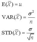
Let the random variables X1,X2,...,Xn be a random sample with E(Xi)= u and VAR(Xi)= s ^2, for i=1,2,...,n. Then

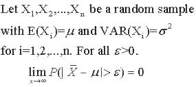
Theorem 2.7-8: Weak Law of Large Numbers
The notion that Xbar gets close to u as the size of the sample increases is the essence of the Law of Large Numbers. The following is the Weak Law of Large Numbers:

 Explore the law of large numbers by using the following applet! Explore the law of large numbers by using the following applet!

Useful Web Resources
Jointly Distributed Random Variables
Jointly Distributed Variables -irving.vassar.edu/faculty/wl/Econ210/joint_prob.pdf

Solutions
Solution to Example 1
If W=(X^2)Y, then E(W)= (1)^2(1)(0.10) + (2^2)(1)(0.25) +(1^2)(2)(0.10) + (2^2)(2)(0.05) =0.1+1+0.2+0.4= 1.7
If W=X(Y^2) then E(W)=(1^2)(1)(0.1)+(1^2)(2)(0.25)+(2^2)(1)(0.1)+(2^2)(2)(0.05)=0.1+0.5+0.4+0.4= 1.4

Solution to Example 2
| x |
0 |
1 |
2 |
| p(x) |
0.15+0.35=0.5 |
0.1+0.1=0.2 |
0.25+0.05=0.30 |
| y |
1 |
2 |
| p(y) |
0.15+0.10+0.25=0.5 |
0.35+0.10+0.05=0.5 |
E(X)=0(0.5)+1(0.2)+2(0.3)=0.8
E(Y)=0(0.5)+1(0.5)=0.5
If W=6X-2Y, E(W)=E(6X-2Y)=6E(X)-2E(Y)=6(0.8)-2(0.5)=4.2-1=3.2
If W=11X+7Y+12, then E(W)=11E(X)+7E(Y)+12=11(0.8)+7(0.5)+12= 8.8 +3.5 +12 =24.3
If W=(X+7Y)/2, then E(W)=[E(X)+7E(Y)]/2= [0.8+7(0.5)] /2= 2.15

Solution to Exercise 2.7-6
A: E(Y)= 0(0.5)+1(0.3)+2(0.15)+3(0.05)=0.3+0.3+0.15=0.75
B: VAR(Y)= (0-0.75)^2(0.5) + (1-0.75)^2(0.3) + (2-0.75)^2(0.15) + (3-0.75)^2(0.05) =0.28125 + 0.01875 + 0.234375 + 0.253125 = 0.7875 = 0.79
C: Y represents the number of computer system crashes in a week. We want the TOTAL number of computer system crashes in a year. This can be expressed by the random variable W, where W=ΣYi where we take the sum of the Yi's for i=1, 2,...,52. Each Yi has the same probability distribution as the random variable Y. Since the number of crashes from week to week are independent, E(W) = ΣE(Yi) for i=1,2,...,52. Since the number of computer system crashes are independent from week to week, ΣE(Yi) = ΣE(Y)= E(Y)+E(Y)+...+E(Y). We add E(Y) 52 times. So our final aswer is
E(W) = Σ E(Yi) = Σ E(Y)= E(Y)+E(Y)+...+E(Y)= (52)(0.75)= 39 for i=1,2,...,52
D: Similarly, VAR(W)= ΣVAR(Yi) = ΣVAR(Y)= VAR(Y)+VAR(Y)+...+VAR(Y)= 52(0.79)= 41.08 for i=1,2,...,52

Solution to Theorem 2.7-4
E(XY)=(1)(1)(0.1)+(1)(2)(0.25)+(2)(1)(0.1)+(2)(2)(0.05)=0.9, and
E(X)E(Y)=(0.8)(0.5)= 0.4
So E(XY) does not equal E(X)E(Y). Therefore, X and Y are not independent.

.
.
|