|
Example 2 |Example 3|Example 4 | Useful Web Resources| Solutions
Theorem 8.2-1:
Central Limit Theorem for Sums. Let X1, X2, ..., Xn be a random sample with E(Xi) = m and STD(Xi)= s for all i. For sufficiently large n, the sum X1 + X2 + ... +Xn has an approximate normal distribution with mean nm and standard deviation s*sqrt(n).
-
Generally speaking, the CLT can be applied with relatively small values of n if the original distribution is symmetric or mound shaped and has very little probablility in the tails of the distribution.
-
If the distribution is skewed as with the exponential, or has heavy tails, then larger values of n are needed for the CLT to apply.
Example 1:
Consider the distribution of the sum of 50 Poisson random variables each of which has mean and standard deviation l=3. The CLT tells us that the sum X= X1 + X2+ ...+ X50 will have an approximate normal distribution with m= nm =50(3)= 150 and s = 3 sqrt(50)=21.2.
P(X £ 140) = P[Z £ (140-150) /21.2 ]
= P(Z £ -0.47)
=1 -F(0.47)
=1-0.6808
=0.3192
 Use the following applet to see how the Central Limit Theorem applies to the Poisson, Bernoulli, Exponential , U-shaped and Uniform Distributions! Help! Use the following applet to see how the Central Limit Theorem applies to the Poisson, Bernoulli, Exponential , U-shaped and Uniform Distributions! Help!

Example 2
Consider the distribution of the sum of 30 Gamma random variables each of which has a=2 and b=3.
Solution
Corollary 8.2-1:
Central Limit Theorem for Sample Means. Let X1, X2, ..., Xn be a random sample with E(Xi) = m and STD(Xi) = s. For sufficiently large n the sample mean Xbar has an approximate normal distribution with mean m and standard deviation s / sqrt(n).
In Theorem 2.7-7 we found that E(Xbar) = m and STD(Xbar) = s / sqrt(n). Moreover, from Theorem 6.2-2 any linear function of a normal random variable has a normal distribution. It follows that if the sum has an approximate normal distribution, then the sample mean will as well.
Example 3:
Let X1, X2, ...., X150 be a random sample with m =50 and s = 7. A sample of 150 is selected at random from this population.
E(Xbar) = m =50
VAR(Xbar) = s / sqrt(n) = 7/sqrt(150) =0.57
P( 45 < X < 55 ) = P[ (45- 50)/7 < Z < (55-50)/7 ]
= P[ -0.71 < Z < 0.71 ]
= 0.5222
Complete the following table:
m |
12
|
25 |
s |
5 |
6 |
n |
100 |
300 |
E(Xbar) |
|
|
STD(Xbar) |
|
|
P( a < X< b) |
|
|
Solution
Example 4:
The normal approximation to the binomial distribution is a special case of the CLT. Suppose X1, X2, ...Xn are independent and identically distributed Bernoulli random variables with probability of success p. Then X= X1 +X2 + ...+Xn is a binomial random variable with
E( Xi ) = p and VAR( Xi ) = p (1-p)
Since X is a sum of a random sample, the CLT asserts that X will have an approximate normal distribution with mean np and standard deviation sqrt [np (1-p) ] for sufficently large n.
The sample fraction Phat= X/n is the sample mean of a random sample of Bernoulli random varibles, so Phat has an approximate normal distribution with mean p and standard deviation sqrt[p (1-p)/n ] .
Example 5:
Suppose the probability that a student has black hair is 0.65. In a group of 100 randomly selected students the probability that more than 50 % have black hair is,
P( Phat > 0.5) = P( Z > [0.5- 0.65] / sqrt [(0.65)(0.35) / 100] )
= P (Z >-3.14)
=1-F(3.14)
=1-0.9992
=0.0008
Suppose the probability that a student owns a car is 0.72. In a group of 300 randomly selected students, what is the probability that more than 75 % own a car?
Solution
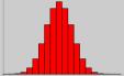 Explore the Central Limit Theorem further by using the following applet! This applet illustrates the CLT using simulated dice-rolling experiments Explore the Central Limit Theorem further by using the following applet! This applet illustrates the CLT using simulated dice-rolling experiments
Applying the Central Limit Theorem
Solutions
Solution to Example 2
The CLT tells us that the sum X= X1 + X2+ ...+ X30 will have an approximate normal distribution with m= nm =nab and s = ab^2 sqrt(n)
A: m = 30(2)(3)=180
B: s = (2)(3^2)sqrt(30)=5.5
C: P(X < 170) = P[X < (170-180)/5.5]
=P( Z £ (-1.82)
=1-P(Z £ 1.82)
=1- F( 1.82)
=1-0.9656
=0.0344
=0.7
Solution to Example 3:
m |
12 |
25 |
s |
5 |
6 |
n |
100 |
300 |
E(Xbar) |
12 |
25 |
STD(Xbar) |
5/sqrt(100) =0.5 |
6/sqrt(300) = 17.3 |
P( a < X < b) |
P( 13 < X < 17 )
= P[ (13- 12)/0.5 < Z < (17-12)/0.5 ]
= P[ 2 < Z < 10]
=0.02275
= 0.0228 |
P(20 < X < 22 )
= P[ (20- 25)/17.3< Z < (22-25)/ 17.3 ]
= P[ -0.29< Z < -0.17]
= 0.0466
|
Solution to Example 5:
P( Phat > 0.75) = P( Z > [0.75- 0.72] / sqrt [(0.72)(0.28) / 300] )
= P (Z >1.16)
=1-F(1.16)
=1-0.8770
=0.123
Help!
When the Web brower is opened, scroll to the bottom of the page until you find a drop down box that says Select Applet. Choose either one of Change sample size only or Change number of samples only and click Open!. When the applet opens choose which distribution you would like to explore. On the right hand side , you can enter in values for the probability/ mean, and the sample size/number of samples. Enjoy!
.
.
|