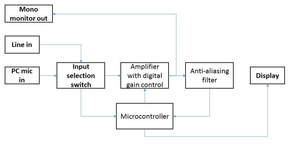
In the last entry I wrote about attempting to understand the bispectrum on an intuitive level by building a piece of hardware to display the bispectrum. It turns out, however, that there are some important mathematical aspects of the bispectrum to take into account in order to best design a system that can acquire a signal and display its bispectrum.
In my first post I plotted a bispectrum. The method I used to calculate the bispectrum, while not incorrect, doesn’t do the bispectrum justice. What I had done to make the plot in my last entry was first calculate the discrete fourier transform F(f) of the signal. Then, at each pair of frequency bins (f1, f2), I multiplied only the magnitudes |F(f1)|, |F(f2)|, and |F*(f1 + f2)| and plotted the result. All this really did is create “hot” (red) spots wherever the product of the signal amplitude is large at each of the frequencies f1, f2, and f1 + f2.
Taking into account the phase of the signal
Taking into account the phase information /_F(f), however, really lets the bispectrum shine. To understand this, we need to look at the definition of the bispectrum (from Wikipedia):
B(f1, f2) = F(f1) F(f2) F*(f1 + f2)
If we take a cue from power spectrum estimation techniques and use Welch’s method to estimate the bispectrum by averaging the complex bispectrum calculated from overlapped windowed segments of the signal, then destructive or constructive interference of the bispectral quantity is possible. This means if we apply the averaging implied by Welch’s method, then the frequency pair (f1,f2) will show up as “hot” on the bispectrum plot when the phase of the sinusoids at each of the three frequencies f1, f2, and f1 + f2 add up to the same constant value over all the windowed segements of the signal. A detailed explanation of how the components can sum or cancel is available on Wikipedia’s page for Bicoherence.
Wait… Bicoherence?
It turns out that if you average a bispectrum in the manner I described above and you normalize it, you’ve actually calculated the bicoherence. Ultimately, however, you’re still calculating a bispectrum. To keep things simple, I will continue to use the term bispectrum rather than bicoherence.
I re-did the plot from my last post with this new approach, as shown below. (For those who are interested, there is 50% overlap between windows 1024 samples long, and a Blackman window applied. Normalization is performed by taking the absolute sum of the bispectra divided by the sum of the absolute bispectra.)
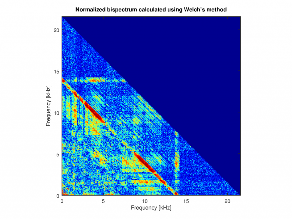
This is certainly different from the previous bispectrum. In fact, all of the hot spots on the previous plot are no longer present in the above plot. This alternate method of averaging many bispectra should be used in the firmware of the Bispectrum Visualizer to take advantage of the phase information present in the signal.