Chapter 10 Multiple regression and interactions

So far, we have only dealt with models with a single predictor. However, often we want to test the effect of multiple predictor variables on a response variable. Multiple regression models include multiple predictor variables, and allows for testing the effect of one predictor while holding all others constant.

10.1 Multiple regression: 2 predictors

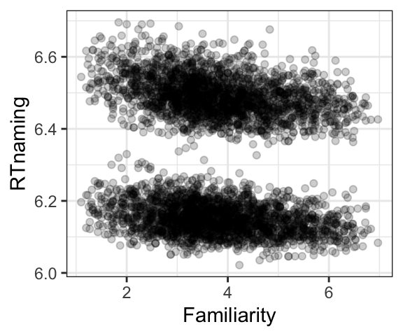
Let’s say you’re interested in how word familiarity predicts naming latency (how quickly it takes participants to say a word out loud). You have the hypothesis that more familiar words will be responded to more quickly. The following graphs are from a dataset built into the languageR package. The data includes listeners’ response times (RTnaming, on a log scale), the familiarity of a word (on a 1 to 7 scale) and the age of the listener (column name AgeSubject, grouped as “old” or “young”).

The plot below shows response time plotted by familiarity. It looks like RT is faster for more familiar words (as predicted). However, probably the more noticeable thing in the graph is the presence of two clusters, one with shorter and one with longer RT, and these clusters don’t seem to be related to familiarity.

require(languageR)
ggplot(english, aes(Familiarity, RTnaming))+geom_point(alpha=.2)

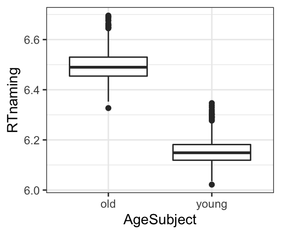
The two clusters indicate that there might be some other systematic factor influencing RT. After thinking awhile, you decide to test whether age might play a role, and decide to plot RT by age, as shown in the plot below. This plot shows that there is a clear effect of age, with younger participants having shorter RTs than older participants.

ggplot(english, aes(AgeSubject, RTnaming))+geom_boxplot()

We can model this joint effect by incorporating both predictor variables into our equation, using the formula below where \(x_1\) is the value of the first predictor and \(x_2\) is the value of the second predictor, and the corresponding \(\beta\) values are the amount that \(y\) will change for every one-unit increase in each predictor.

\[ \begin{aligned} One\ predictor: y &= \beta_1x+\beta_0\\ Two\ predictors: y &= \beta_1x_1+\beta_2x_2+\beta_0 \end{aligned} \]

We can build a linear regression model including both predictors by simply including both in the formula:

mdl = lm(RTnaming ~ Familiarity + AgeSubject, english)

In the corresponding output, the rows in the Coefficients table corresponding to the two predictors will give us information about the effect of each predictor separately. Familiarity has an estimate of about -0.01, indicating that for every 1-unit change in familiarity, there is a 0.01 second decrease in response time. This number seems tiny, but the small p-value indicates that it is a reliable effect. The estimate for Age is about -.34. Since Age is a categorical factor, this estimate corresponds to the difference between old and young participants. It shows that younger participants have a response time of -.34 less than older participants, and this is also significant. Overall, we can conclude from this: Both familiarity and age have a significant effect on response time: response time decreases for more familiarity words (with an 0.0147 decrease in response time a 1-unit increase in familiarity), and younger participants respond faster (by -0.34 on average) than older participants.

## 
## Call:
## lm(formula = RTnaming ~ Familiarity + AgeSubject, data = english)
## 
## Residuals:
##       Min        1Q    Median        3Q       Max 
## -0.155235 -0.032830 -0.002964  0.030688  0.197551 
## 
## Coefficients:
##                   Estimate Std. Error t value Pr(>|t|)    
## (Intercept)      6.5493734  0.0025632 2555.20   <2e-16 ***
## Familiarity     -0.0147206  0.0006208  -23.71   <2e-16 ***
## AgeSubjectyoung -0.3419891  0.0014268 -239.69   <2e-16 ***
## ---
## Signif. codes:  0 '***' 0.001 '**' 0.01 '*' 0.05 '.' 0.1 ' ' 1
## 
## Residual standard error: 0.04822 on 4565 degrees of freedom
## Multiple R-squared:  0.9271, Adjusted R-squared:  0.927 
## F-statistic: 2.901e+04 on 2 and 4565 DF,  p-value: < 2.2e-16

We can write the formula for the model as follows, if we sub in the estimates from the coefficients table for the values for the effects of familiarity, age, and the intercept respectively:

\[ \begin{aligned} y &= \beta_1x_1+\beta_2x_2+\beta_0 \\ y &= (-0.0147206 \times Familiarity)+(-0.3419891 \times Age)+6.5493734 \end{aligned} \] A graph of the predicted values is shown below.

We can then, if we want, get the predicted values for this model by substituting relevant values for Familiarity and Age in the formula. Remember that a 2-level categorical variable like age is coded as 0 for the first level and 1 for the second. So if we wanted to predict the response time for a word with familiarity 5 by a younger speaker, we would plug in 5 for familiarity and 1 for age. For an older speaker, we would plug in 5 for familiarity and 0 for age. The predicted response times for each of these are shown below; you confirm that these match up with the predicted lines in the graphs above.

## [1] 6.134281

## [1] 6.47627

Note that in this model, the predictors are modeled as independent: The predicted effect of familiarity is the same for both younger and older speakers, and the effect of age holds regardless of the level of familiarity. In this case, based on the graph, this seems like a reasonable model of the data. However, in other situations, as we will see below, the effect of one predictor may be different depending on the value of the other predictor, and we will want to be able to include that information in our model. We can do this using interactions.

10.2 Interactions

In many situations where there are multiple predictor variables, the effect of a given predictor variable depends on the value of a different predictor variable. The models we have looked at so far do not allow for this possibility; rather, they make the best prediction they can assuming that the effect of each predictor variable is the same, regardless of the value of the other variable. Including an interaction between predictor variables in our linear model allows us to quantify and test the extent to which the effect of one predictor variable might differ depending on the value of another predictor variable.

The example below deals with the question of how children’s accuracy in producing correct Englihs verb forms varies based on two predictor variables: 1) verb regularity (whether the verb is regular or irregular) and 2) age. The (hypothetical) dataset below includes children’s percentage accuracy in use of verb forms for a set of younger and older children, in verbs that are either regular or irregular.

Outcome variable: % accuracy
Predictor variable 1: Age (younger vs. older)
Predictor variable 2: Verb Regularity (regular vs. irregular)

We can ask the following questions related to each predictor:

Age: Does accuracy differ based on age (older vs. younger)?
Regularity: Does accuracy differ for regular vs. irregular verb forms?

We can also ask whether the effect of one predictor differs based on the value of the other predictor. There are actually two ways to ask this; both are accurate!

Does the age effect differ for regular vs. irregular verbs?
Does the regularity effect differ for younger vs. older children?

First, let’s look at the outcome variable plotted by each of the predictor variables separately. The first plot below shows the effect of age: it looks like on average, older children are more accurate than younger children. The second plot shows the effect of regularity: on average, irregular verbs have higher accuracy than regular verbs.

We can confirm the direction and significance of these effects with a multiple regression model including both predictor variables.

Based on this model and the estimates, we might make the following interim conclusions:

Older children have significantly higher accurate than younger children (by about 27%).
Irregular verbs are significantly more accurate than regular verbs (by about 21%).

## 
## Call:
## lm(formula = accuracy ~ age + regularity, data = vb.dat)
## 
## Residuals:
##     Min      1Q  Median      3Q     Max 
## -31.049 -16.652   1.414  16.245  35.475 
## 
## Coefficients:
##               Estimate Std. Error t value Pr(>|t|)    
## (Intercept)     39.782      3.482  11.425  < 2e-16 ***
## ageold          27.282      4.021   6.785 2.11e-09 ***
## regularityirr   21.121      4.021   5.253 1.29e-06 ***
## ---
## Signif. codes:  0 '***' 0.001 '**' 0.01 '*' 0.05 '.' 0.1 ' ' 1
## 
## Residual standard error: 17.98 on 77 degrees of freedom
## Multiple R-squared:  0.4888, Adjusted R-squared:  0.4755 
## F-statistic: 36.82 on 2 and 77 DF,  p-value: 6.026e-12

However, what if we plot the data broken down by both factors? Take a few minutes to make your own interpretations of the graph in terms of our questions. What is the effect of age, and what is the effect of regularity?

Let’s re-examine our conclusions from above:

Older children are more accurate than younger children. However, when broken down by regularity, older children only seem to be better than younger children for regular verbs. For irregular verbs, the groups are about the same, and if anything older children are less accurate than younger children!
Irregular verbs are more accurate than regular verbs. Again, this statement does not hold overall; it depends if we’re looking at older or younger children. Younger children show higher accuracy for irregular verbs, but older children show the opposite pattern.

Because of this, the conclusions from the regression model above do not really give an accurate picture of the data. That’s because in the formula, the effect of each predictor is fixed and independent of the value of the other predictor. However, we can add an interaction to the model, by adding an additional coefficient that models the joint effect of the two predictors. The coefficient \(\beta_3\) will tell us how much the effect of one predictor variable changes for every one-unit change in the other predictor variable.

\[ \begin{aligned} One\ predictor: y &= \beta_1x+\beta_0 \\ Two\ predictors: y &= \beta_1x_1+\beta_2x_2+\beta_0 \\ Two\ predictors\ plus\ interaction: y &= \beta_1x_1+\beta_2x_2+\beta_3x_1x_2+\beta_0 \end{aligned} \]

We can include an interaction in our linear model by simply combining the two variables with * instead of +:

mdl.interact = lm(accuracy ~ age * regularity, vb.dat)

## 
## Call:
## lm(formula = accuracy ~ age * regularity, data = vb.dat)
## 
## Residuals:
##      Min       1Q   Median       3Q      Max 
## -15.6614  -7.8286   0.3447   6.5412  20.0873 
## 
## Coefficients:
##                      Estimate Std. Error t value Pr(>|t|)    
## (Intercept)            24.395      1.979   12.32   <2e-16 ***
## ageold                 58.057      2.799   20.74   <2e-16 ***
## regularityirr          51.896      2.799   18.54   <2e-16 ***
## ageold:regularityirr  -61.549      3.959  -15.55   <2e-16 ***
## ---
## Signif. codes:  0 '***' 0.001 '**' 0.01 '*' 0.05 '.' 0.1 ' ' 1
## 
## Residual standard error: 8.853 on 76 degrees of freedom
## Multiple R-squared:  0.8777, Adjusted R-squared:  0.8729 
## F-statistic: 181.8 on 3 and 76 DF,  p-value: < 2.2e-16

You will notice that there is now an additional line in the Coefficients table, and this corresponds to the interaction term. There is an estimate of about -61, and this effect is significant. We will walk through the numerical interpretation of this below. However, the most important thing to note is that when there is a significant interaction, the effect of one predictor differs depending on the value of the other predictor. This means that even though you see significant effects for Age and Regularity separately in the coefficients table, these values are not necessarily meaningful, because they are not consistent across the full set of data.

So what do we do if we want to answer our question? First, we need to note that there was a significant interaction; that the effect of verb regularity differs depending on the age of the child: that younger children show lower accuracies for irregular vs. regular verbs, but older children are more accurate for regular verbs. It would also be good to report the mean values to give a sense of the size of the effect.

You might then also want to know whether those differences are actually significant (i.e. is there really a meaningful difference between regular and irregular verbs for older children?). There are multiple ways to test this. It is in some cases possible to test these questions directly in the model, but other times it is necessary to run what follow-up tests to determine significance. One simple way to do this is simply to split the data up by age so that you have two datasets, then run a simple linear regression testing the effect of regularity on each (note that this is usually not the most statistically sound thing to do, but it will give a general idea).

Numerical interpretation of the interaction coefficient

Here we will walk through details of the the numerical interpretation of the coefficient table. The model coefficients are all repeated below, as well as the plot of the data so you can confirm the values. All values are rounded to the nearest whole number for discussion.

##                       Estimate Std. Error   t value     Pr(>|t|)
## (Intercept)           24.39467   1.979499  12.32366 8.396131e-20
## ageold                58.05713   2.799434  20.73888 5.062392e-33
## regularityirr         51.89570   2.799434  18.53793 6.357441e-30
## ageold:regularityirr -61.54926   3.958997 -15.54668 2.582520e-25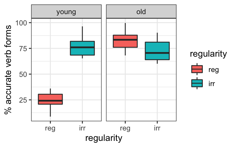

The estimate for the intercept (24) represents the average accuracy when both predictors are at their reference level (younger, regular). This means that younger children have an average accuracy of 24% for regular verbs.
The estimate for age (58) represents the effect of age (i.e. the difference between older and younger children’s accuracy) for verbs at the reference level (i.e. regular verbs). In other words, older children have 58% higher accuracy for regular verbs than younger children, which, as we know from the intercept, is 24. So older children have \(24+58=82\%\) accuracy for regular verbs.
The estimate for regularity (52) represents the effect of regularity (i.e. the difference between irregular and regular accuracy) for children at the reference level for age (i.e. younger children). Since we knew that younger children had 24% accuracy for regular verbs (intercept), this tells us that younger children have \(24+52=76\%\) accuracy for irregular verbs.
So far, we have three predicted values: Younger/Regular, Older/Regular, and Younger/Irregular. What we’re missing is the predicted value for older children using irregular verbs.
We can obtain this using the estimate for the interaction (-62). We can interpret in two different ways, but as you will see, they are mathematically equivalent, so we will end up with the same answer!
- The effect of age is 62 less for irregular than for regular verbs. Since we knew that the effect for age was 58 for regular verbs, the effect for age for irregular verbs will be \(58-62=-4\). Since we found above that younger children have 76% accuracy for irregular verbs, older children have \(76-4=72\%\) accuracy for irregular verbs.
- We can also frame this in a different way, and say that the effect of regularity is 62 less for older than for younger children. Since we know that the effect of regularity was 52 for younger children, the effect of regularity for older children will be \(52-62=-10\). Since we know that older children had an accuracy of 82% for regular verbs, this means that their predicted accuracy for irregular verbs is \(82-10=72\%\) for irregular verbs.