Chapter 7 Statistical hypothesis testing
Statistical inference is the process of determining how confident we are that the properties of our sample data reflect the broader population. We have seen that our confidence can be influenced by the variance and the size of our sample, and how we can use confidence intervals to calculate ranges of plausible population parameters based on our sample data.
This section introduces the concept of statistical significance, which allows us to make binary statements about whether the patterns we see in our data are “meaningful”, such as:
- VOT of voiceless stops is significantly longer for German than for French speakers.
- The frequency of the discourse marker “like” in English is changing significantly across generations.
- The emotional valence of a word has a significant effect on response time.
- There is a significant correlation between use of an L2 and age of acquisition.
This section discusses the concept of Null Hypothesis Significance Testing (NHST), the most common basis for testing statistical significance2.
7.1 Null Hypothesis Statistical Testing
We’ll walk through this conceptually using an example. Let’s say we’re interested in whether VOT of Korean aspirated stops is changing over time. We have the average VOT values for a group of younger speakers and a group of older speakers, both from Seoul. In our sample, younger speakers have shorter VOTs than older speakers, by 17ms on average (boxplots are shown below, with the purple asterisk representing the mean). We want to be able to make a statement about whether we can infer that this age-based difference holds in the broader population: Is there a significant difference between the VOT of younger vs. older speakers?

The way we do this is a little counter-intuitive. We won’t actually be directly testing the plausibility that there is a 17ms difference between older and younger speakers in the broader population. Instead, we will be testing the plausibility that there is no difference between younger and older speakers in the broader population. If we can reject the possibility that there’s no difference, we will conclude that there is a significant difference between younger and older speakers (but we actually can’t conclude anything about how big that difference is; just that there is one!).
Here’s the overall procedure on a high level, which we will then work through with specific examples.
- Construct a null hypothesis \(H_0\). This is a statement about the broader population that we would find useful to disprove in order to say something we want to say about the data. In this case, since we’re interested in whether there is a difference, our null hypothesis would be that there is no difference between the age groups in the broader population. More precisely, we can state this as the difference in average VOT between older and younger speakers is zero.
- Formulate the alternative hypothesis \(H_a\). This is the set of all possible scenarios that NOT the null hypothesis (you can think of the null and alternative hypotheses as being in complementary distribution. ❤Phonology❤). In this case, the alternative hypothesis is that there is a difference in age groups (or the difference in VOT between older and younger speakers is not zero).
- Then, we conduct a statistical test to ask: Is the null hypothesis within the plausible range of what we could expect, given the properties of our sample and what we know about inference?
- If it is not plausible, we reject the null hypothesis. This means that it’s very unlikely there is no difference between the two groups in the general population, so we can conclude that there is a significant difference between groups.
- If the null hypothesis is plausible, we cannot reject the possibility that there’s no difference between groups, so we say that the difference between the groups is not significant.
- Note that even if we can’t reject the null, we also can’t prove it’s true! We can never prove that the groups are the same, we can only say we don’t have evidence that they are different.
| Null hypothesis (\(H_0\)): | No difference in age groups | \(H_0: \mu_{older} - \mu_{younger} = 0\) |
| Alternative hypothesis (\(H_a\)): | Difference in age groups | \(H_a: \mu_{older} - \mu_{younger} \neq 0\) |
7.1.1 Significance thresholds and p-values
OK, but how do we actually make the decision about what is plausible or not? This decision is based on a value called the t-statistic, which is calculated taking into account the values in the sample data, the variance, and the sample size. The t-statistic is incorporated into many common statistical tests, including the one we will be using, linear regression.
A large absolute value for \(t\) indicates a lower probability that we would see this data if the null hypothesis were true. \(t\)-values with absolute values greater than 2 generally mean that probability of this sample occurring if the null were true would be less than 5%.
With the help of R, we can compute the exact probability, and this is called the p-value. You can think of the p-value as the probability of seeing the data if the null hypothesis were true. A very small value of \(p\) means that it would be very unlikely to see this sample of data if the null were true, and we can therefore reject the null as implausible.
By convention, the cutoff for statistical significance is for p-values of less than .05. In other words, if we have a p-value of less than .05, we reject the null hypothesis. If, as in this case, the null hypothesis was that there was no difference between two groups, then we can conclude that the difference between groups is significant when \(p<.05\).
We will not go into the details of how \(t\) and \(p\) are calculated (R will do this for you), but it is not too hard to understand if you understand the logic of 95% confidence intervals! You can find a good discussion of the t-statistic in Winter (2019), Chapter 10.
7.1.2 Error
We want to be certain about the conclusions we draw: after all, that is the whole point of doing statistics!
In the real world, the null hypothesis is true or false:
- True: there is no difference between the groups in the real world
- False: there is a difference between groups in the real world
Usually, there’s no way to test whether this is actually true, which is why we are doing inference. We use our statistical tools to determine whether we can plausibly reject the null hypothesis. We hope that we (correctly) reject it when it’s false, and that we (correctly) don’t reject it when it’s true. However, we can never be truly sure, and there is always the possibility for error. This error can be of two different types, as shown in the table below.
| Stats: reject \(H_0\) | Stats: don’t reject \(H_0\) | |
|---|---|---|
| Real life: \(H_0\) is true | Type 1 error | correct decision |
| Real life:\(H_0\) is false | correct decision | Type 2 error |
One possibility, called Type 1 error, is when we reject a null hypothesis when it is actually true. In other words, there is no difference between groups in the real world, but we incorrectly conclude that there is a difference. The significance threshold is designed to control the rate of these types of errors: for a significance threshold of .05, there is a 5% chance that we would incorrectly reject the null. This means that for 1 out of every 20 tests, we might expect to see a “false positive” where we reject the null hypothesis, and conclude that a difference is significant, even when it’s not!
Type 2 error occurs when we fail to reject the null hypothesis even when it is actually false. In other words, there actually is a difference between groups in the real world, but do not reject the null (i.e. we do not see evidence of a significant difference). There are many reasons this can occur, but is often because the experiment doesn’t have sufficient power: the sample is too small, or has too much variability, or the effect itself is too small, for a significant effect to be detected.
7.1.3 Working through the logic of NHST with confidence intervals
The last chapter included an example of how to make inferences with confidence intervals. Here we will revisit the same example, but we will frame it in terms of NHST. The logic is exactly the same as it was explained in words. This is just a way of formalizing the logic.
The example was asking question of whether students’ test scores have changed over time. Our sample is a distribution of current scores (we’ll consider two different possible scenarios, just for the sake of comparison: Scenario A and Scenario B), and we know the value of scores in the past (70). We want to know: Is the average current test score significantly different than 70?
The 2 hypothetical distributions of current scores, Scenario A and Scenario B, are shown below, plotted with the 95% confidence interval for each. The dashed line shows 70.
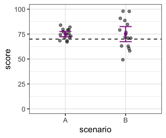
We know that (in both scenarios), the average current score is 75. We know that the current score in our sample is higher than 70. What we want to know is: can we infer that this difference between our sample and the comparison value is reflective of the broader population?
Since we are interested in whether the mean score for current students (\(\mu_{current}\)) in the broader population is different than 70. We want to set up a null hypothesis that there is no difference (i.e. that the current score is 70), and try to disprove that. The alternative hypothesis would be that the current score in the population is not 70.
\[ H_0: \mu_{current} = 70 \\ H_a: \mu_{current} \neq 70 \] The next step is to use tools from statistical inference ask: Is the null hypothesis within the plausible range of what we could expect, given the properties of our sample? In this case, we already have the tools we need to answer that. If we consider the “plausible range” to be 95% confidence, then our 95% confidence interval gives us the range of plausible population means.
Scenario A: If our data were as shown in Scenario A, we can see that 70 is not within the confidence interval, and therefore not within the plausible range of current population means. Based on this:
- we reject the null hypothesis that the current mean is 70.
- we accept the alternative hypothesis that the current mean is not 70.
- we can say that the average current test score is significantly different than 70.
- we can conclude that test scores are likely changing over time.
Scenario B: If our data were as shown in Scenario B, 70 is within the confidence interval. Therefore, 70 is one plausible value for the current population mean. Based on this:
- we cannot reject the null hypothesis that the current mean is 70.
- we would conclude that the average current test score is not significantly different than 70.
- note that we cannot conclude that the null hypothesis is true, or that the current average is 70!
- all we can say is that there’s not enough evidence to show that there is a difference.
- We cannot conclude that test scores are changing over time (but we also can’t conclude they are the same!).
If the conclusions from the second scenario seem rather unsatisfying, you’re not alone! When using NHST, it’s hard to make any conclusive statements when you fail to reject the null hypothesis. Because of this, when using NHST it’s important to try to set up your questions in a way that will give interpretable answers. Specifically, you will never be able to conclude that two things are the same: you will only be able to make conclusions about differences.
7.2 Statistical tests
OK, but we still haven’t talked about how to do the actual tests! NHST can be incorporated into many different kinds of statistical tests. If you have taken an intro stats course, or talked to people who have, you might be familiar with a bunch of different kinds of tests, all for different kinds of data:
| test | description |
|---|---|
| one-sample t-test | compare a distribution of continuous data to a single value |
| independent samples t-test | compare two distributions of independent continuous data |
| paired t-test | compare two distributions of paired continuous data |
| chi-squared test | compare distributions of a categorical variable |
| ANOVA | account for predictors with more than 2 levels, consider multiple predictors at once |
It turns out that these are all special cases of a linear model, and in this course, we are going to consider them all as such. The math is the same, and the results are the same. It takes a little more work to understand up front, but the good news is, you don’t have to learn a bunch of different tests and when to use them!
If you are interested in learning more about how these specific tests are special cases of linear models, this link and Appendix A of Winter (2019) are good resources!