Chapter 6 Samples, Populations, and Confidence Intervals
For a more thorough but still highly accessible introduction to the concepts introduced here, I recommend Navarro (2018), Chapter 10.
As we have seen, descriptive statistics allow us to describe patterns in our data. Inferential statistics gives us tools to test how likely it is that these descriptive patterns are representative of the broader population, as opposed to a quirk of the specific data we collected.
Before going into the details, we will start with an example to show how this works intuitively. Let’s say you’re struggling with a university course, and you see an ad for a tutoring service. The tutoring service claims that based on a controlled study, students who completed the course scored on average 10 points higher on the final exam than students who did not. You’re considering the course, but you only want to spend your time and money if you’re pretty sure that the tutoring is actually likely to be effective, and you look into the data. Below are four hypothetical sets of final exam scores from two groups of test-takers who have or have not completed the tutoring course. Based on each of these scenarios, how confident would you be that that there is a systematic difference between test scores for students who have vs. have not taken the tutoring course, beyond this specific sample and in the broader population?

We can calculate the summary statistics of these samples and find that in all of the examples, the Tutor group has a higher mean test score than the NoTutor group, as claimed by the tutoring service (the difference in means between the two groups is the “diff” value given in the plots). However, in any real-world situation where you are looking at samples of data, it is almost always the case that there will be differences between sample means - it is highly unlikely to come up with the exact same number, even if there is actually no difference between the groups in the real world. So how do we assess whether this difference is “meaningful” or likely to be a “real” difference?
Looking at the examples above, you likely have some intuitions about how confident you are that these differences are real. For Dataset 1, although there is an 11 point difference in the means across the two groups, there’s also a large range of individual variation and not a lot of data points, so it seems fairly likely that the average difference between groups might just be driven by the specific points in this dataset. Now compare the other three datasets to Dataset 1. Dataset 2 actually has a smaller difference between the two groups, but most people share the intuition of more confidence that there is a real difference between the groups, and this is because the range of individual variation is smaller. For Dataset 3, the means and ranges are the same as Dataset 1, but there are more datapoints, which usually instill more confidence that we can trust the sample. Finally, Dataset 4 has the same range and number of datapoints as Dataset 1, but the overall difference is larger, again making us more confident that the difference we see in the sample is likely to reflect a difference between the groups in the real world.
To sum up, our intuitions about how confident we can be about generalizing differences found in a specific dataset to the real world are influenced by three things:
- Difference in means across groups
- Amount of dispersion/variation
- Sample size (number of datapoints)
These same three “ingredients” form the basis of the formulas that are used in inferential statistics, allowing us to quantify how confident we can be that the patterns in a sample generalize to the larger population.
6.1 Population vs. Sample
When testing linguistic questions, we usually don’t have the full possible dataset to use as a test case. Instead, we have a sample, or subset of the population, and use the patterns we see in this sample to make generalizations about the larger population.
Population
Defining a statistical population is a bit trickier than it may initially seem. The population is the full set of relevant data points to which we would like to generalize. What counts as relevant, and therefore what counts as a population, depends on the research question.
For example, even considering the same outcome variable (VOT), the population of interest can differ based on the research question:
| Research question | Population |
|---|---|
| Does VOT differ for European vs. Quebec French speakers? | All speakers of Quebec and European French (one average VOT value per speaker) |
| Doe VOT differ for words beginning with /p/ vs. /k/? | All linguistic items beginning with /p/ or /t/ (one average VOT value per word) |
| Does VOT differ for languages that have more vs. complex morphological structure? | All languages (one average VOT value per language) |
Note that populations in this sense:
- can be finite and measurable (the number of languages spoken by of all residents of the GTA)
- can be infinite and hypothetical (speaking rate of all sentences of English)
- do not have to be made up of people!
Sample
The sample is the actual dataset you have - the result of a single experiment or study - and a subset of the population you would like to generalize to. It is important that the sample be as representative as possible. This means that it is balanced with respect to relevant aspects of the population.
Example: Let’s say you are interested in examining the distribution of number of languages spoken by Ontario residents. If you take a survey of a sample of university students living in Mississauga, this is not necessarily representative because it is likely that number of languages spoken differs systematically by geographical region, age, and likely other factors. To make this a representative sample of the population of Ontario, you would need to expand your sample to include other geographical regions and age ranges. Alternatively, you can keep the narrow sample, but in this case the population you can generalize to will be the number of languages spoken by UTM students (instead of Ontario residence).
It is never possible to have a completely representative sample, since each individual member of the population (whether it is a word or a person or anything else) will likely have its own unique characteristics (and by definition, your sample is not going to include every member of the population, so you’ll always be missing out on some!). Nevertheless, it is important to think about factors that may affect your measurements, and make thoughtful decisions about which members of the population to include in a way that is as representative as possible given your resources.
6.2 Generalizing from sample to population
We have defined a population (a hypothetical set of all relevant values) and a sample (a specific subset of those values). What we are really interested is the properties of the population, but since we don’t have data from the full population, the best we can do is make inferences based on our sample. We can calculate summary statistics, such as mean and standard deviation, of the sample. We then do a little math to quantify how confident we can be that the sample statistics are good estimates of the general population.
We’ll be talking about means and variances of the sample, and means and variances of the population. To keep straight which is which in formulas, Roman letters to refer to parameters of a sample, and Greek letters are used to refer to parameters of the hypothetical population, as shown below (these are standard conventions).
| sample | population | |
|---|---|---|
| Definition | The data we have | What we want to generalize to |
| mean | \(\bar{x}\ or\ m\) | \(\mu\) |
| standard deviation | \(s\) | \(\sigma\) |
| sample size | \(n\) |
To foreshadow how properties of the sample will affect our confidence in its reliability:
- Larger samples provide better estimates than smaller samples.
- Samples with less dispersion/variability provide better estimates than samples with more dispersion/variability.
We’ll walk through the logic of how this works in the the following section.
Sampling distribution (or: simulating thousands of experiments)
Let’s work backwards for a bit. Usually, when we’re doing research, we have a sample and we want to generalize about a population…so we don’t know the parameters of the actual population. But what if we actually did know what the population was? If we take a random sample from this population, how likely is the mean of the sample to be close to the mean of the population? We can look at this by simulating a bunch of random samples from the population, taking the mean of each, and looking at the distribution of these means. This is called the sampling distribution.
You can think of the sampling distribution as the results of a bunch (like, thousands!) of mini-experiments done in a hypothetical world. By looking at this distribution, we can get a sense of how reliable one mini-experiment, or one sample, is likely to be. It turns out that reliability is affected by 1) how big the sample is for each mini-experiment and 2) how variable the population is. This makes sense intuitively, but we’ll show it below, using an example (and figures) from Navarro (2018) (Chapter 10).
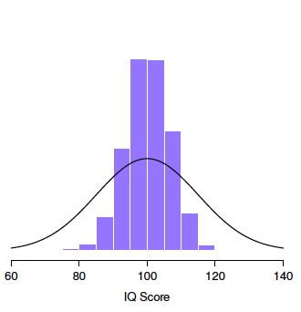
We’ll be looking at IQ scores: IQ tests are standardized to have a mean of 100 and a standard deviation of 15, so unlike in most experiments, we actually know the true parameters of this population. Here’s what we’re going to do:
- Population: The full set of IQ scores (with mean 100 and standard deviation 15)
- Compute the sampling distribution of a series of 10,000 mini-experiments
- 1 mini-experiment:
- Take 1 sample of size n
- Compute the mean of the sample
- Then do the same thing 9,999 more times!
- You’ll end up with 10,000 means (one for each experiment)
- Plot a histogram of the distribution of these 10,000 means
- 1 mini-experiment:
- We can do the same thing, but using different sample sizes, or different values of n.
To give an example (taken from Navarro (2018)), below are the results of the first 10 mini-experiments (or Replications) for a sample size of 5. There would be 10,000 replications in total - these are just the first 10. For each mini-experiment, there is a sample mean. The histogram shows the plot of all 10,000 sample means, or the sampling distribution. This is overlaid with a density plot showing the distribution of the population. You can see that the sampling distribution is narrower (i.e. has a smaller standard deviation) than the population distribution: more of the values are clustered around the true population mean.

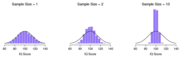
Effect of sample size on the sampling distribution
It turns out that the variance of the sampling distribution is directly connected to the sample size. The figure below shows sampling distributions from simulations of 10,000 experiments with sample size 1, 2, or 10. The variance of the distribution decreases as the sample size gets larger. Another way to think about it is that with larger sample sizes, the values are closer to the population mean…which means that larger sample sizes lead to better estimates of the population. In other words, we can be more confident that our sample mean is close to the population mean when we have larger samples!
Effect of variability on the sampling distribution
We saw above that sample size affects our confidence in the sample mean, with larger samples giving greater confidence that the sample mean is representative of the population mean. The dispersion/variability of a population also affects how much confidence we will have in the sample mean: populations with greater variability will result in more variable samples, and a more variable sampling distribution. However, as the sample size gets larger, the shape of the sampling distribution will become narrower and will converge on the mean of the population.
Sample to population: summing up
In the previous section, we performed simulations of thousands experiments by pulling thousands of samples from a hypothetical population with a known mean and variance, resulting in sampling distributions.
These sampling distributions have several important properties:
- They follow a normal distribution
- Their mean is identical to the population mean
- Their variance is influenced by the sample size and population variance: Specifically, the standard deviation of a sampling distribution, also called standard error or SE, can be calculated by the following formula, where \(\sigma\) is the standard deviation of the population and n is the sample size:
\[ SE\ (standard\ error) = \frac{\sigma}{\sqrt{n}} \]
These simulations show us that our confidence in how good an estimate the sample mean is of the population mean depends on the sample size (with larger samples giving better estimates) and the population variability (with less variability giving better estimates).
In real-life research, we don’t know the characteristics of the population (that’s what we’re trying to find out!). Instead, we just have a single sample. However, the information from this sample, combined with what we have learned about the properties of sampling distributions from these simulations, we can actually come up with a reasonable range of estimates for the parameters of the population. We do this with confidence intervals.
6.3 Confidence intervals (CIs)
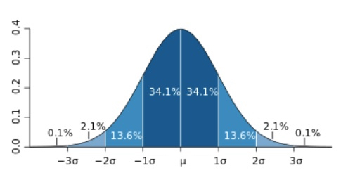
Sampling distributions follow a normal distribution. The shape of normal distributions is fixed such that we can calculate the percentage of density of data that lies under the curve at each point; for example, about 68% of the data falls within 1 standard deviation of the mean, and 95% falls within 1.96 standard deviations. This will be the case for ANY normal distribution, regardless of its variance (we are not covering why this is the case here, but you can find more discussion in Navarro (2018), among other sources).
Because sampling distributions are normally distributed, if we have an estimated sampling distribution, we can calculate a “confidence interval” (CI), or the range of values we would expect to contain the population mean 95% of the time if we did many many experiments.
But we don’t know the actual sampling distribution because we don’t know the properties of the actual population! This is true. We therefore estimate the parameters of the sampling distribution of the population based on the sample parameters - it’s not perfect, but it’s our best guess!
Why 95%? We use the example of a 95% confidence interval because that is most standard, but it is possible to do this for any percentage confidence.
6.3.1 Calculating confidence intervals
To calculate a CI for a sample (i.e. any distribution of data), we need to know three things about the sample:
- The sample mean \(m\)
- The sample standard deviation \(s\)
- The sample size \(n\)
With this information, we can calculate the boundaries of the 95% interval using the following formula (using plus for the upper bound and minus for the lower bound):
\[ CI_{95} = m \pm (1.96 \times SE) \] …which is the same as:
\[ CI_{95} = m \pm (1.96 \times \frac{s}{\sqrt{n}}) \]
Calculating confidence intervals by hand
We will first calculate a CI by hand (…with the help of R…), returning to our example of test scores from earlier in this chapter.
## [1] 76 81 73 77 44 64 51 82 59 77We can calculate the 95% boundaries as follows (note that length(scores) will give the length of the vector, which is equivalent to \(n\), the number of samples):
## [1] 60.19709## [1] 76.60291Therefore, based on this sample, our 95% confidence interval as an estimate for the mean test score in the population is between about 60 and 77.
Note that CIs refer to our confidence about the mean of a population! This does not mean that we don’t expect to see values outside of it: we definitely do (and those occur in our sample). The CI provides information about the values we can expect to represent the average value of the population.
Influences on confidence intervals
There are three pieces of information about the sample that go into the CI calculation: the sample mean, sample standard deviation (variance), and sample size. Therefore, these are all going to affect the CI. The way each affects it is pretty intuitive.
- Sample mean: The sample mean will always be the center of the confidence interval, so CIs of distributions with different means will have different centers.
- Sample standard deviation: Confidence intervals will be wider (i.e. less precise) for samples with higher standard deviation.
- Sample size: Confidence intervals will be narrower (i.e. more precise) for larger samples.
These last two follow the ideas discussed at the beginning of this section, intuitivey, and in the discussion of sampling distributions: we expect samples with less variability (i.e. a tighter distribution) to provide better estimates, and we expect larger samples to provide better estimates.
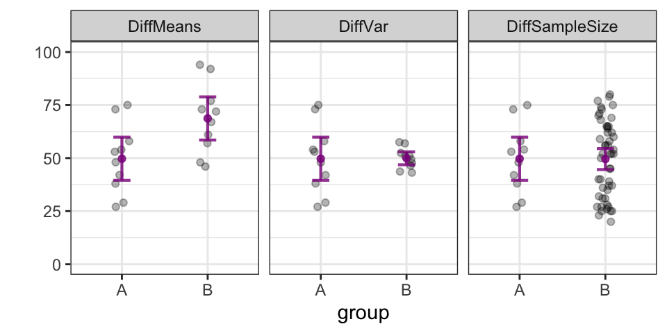
The figure below provides a visual depiction of how the 95% confidence intervals are influenced by these three factors. The lines show the 95% confidence interval for each distribution of grey points. Distribution A is the same across all three panels. Distribution B differs from A in its mean in the first panel, in its variance in the second, and in its sample size in the third.
6.3.2 Making inferences based on confidence intervals
We can practice using confidence intervals to make inferences about what the overall value is likely to be. Let’s say that a linguistics professor in 1967, when UTM (then Erindale College, honestly it doesn’t look much different) opened its doors, designed a final exam such that the average score of the students was 70%. The same exam is given today, and you have the distribution of scores from the class of 2022. The average score was higher: 75%. You’re wondering whether this difference is actually meaningful - how confident can we be that students are actually doing better? We can use confidence intervals to help us decide. The properties of the distribution are going to affect our decision.
Let’s consider a couple possible 2022 scenarios, for the sake of comparison. There are 2 distributions, A and B, both of which have a mean of 75%. The data is shown below, as well as the 95% confidence intervals. Our question is: is there good evidence to believe that the average score in 2022 is different than 70% (shown on the figure by the dashed line)?
## [1] 67 68 68 72 72 73 74 75 75 77 79 79 80 82 84## [1] 49 58 61 63 63 71 71 72 77 79 85 89 91 98 98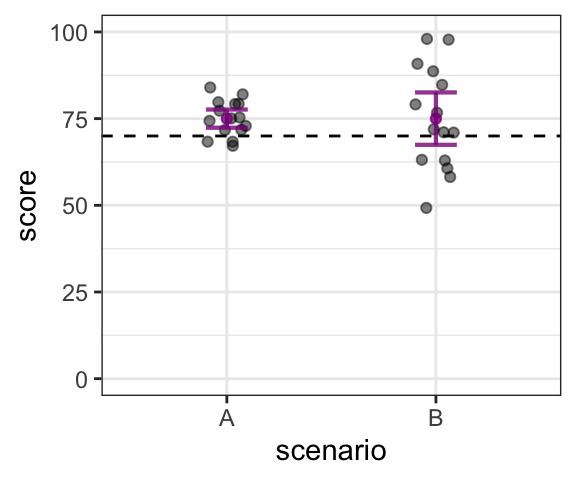
Again, in both Scenarios A and B, we are looking at distributions that have a mean of 75. In Scenario A, the 95% confidence interval does not include a score of 70 (even though some individual scores are below 70). This means that we can be fairly confident that 70 is not within the range of plausible mean values for students in 2022; in other words, we can infer that students in 2022 have systematically higher scores than those in 1967. On the other hand, in Scenario B, the confidence interval does include a score of 70. This means that 70 is among the range of plausible mean values for students in 2022, and we cannot conclude that there is any systematic difference in scores between students in 2022 and 1967.
To sum up, when trying to determine whether the mean of a distribution is likely to be different than a specific value, we cannot just count on the size of the difference between the sample mean and the specific value (in this case, a score of 75 vs. 70). The size of the difference will have an effect: for example, if the new mean was 85, not 75, such that all the 2022 scores were 10 points higher, the confidence intervals would also be 10 points higher, and in this case, both scenarios would exclude the value of 70. However, this example shows that even when the amount of difference is the same, the variance and size of the sample will also affect our decision.
Evidence of lack of difference \(\neq\) evidence of being the same!
One very important thing to note is that even though, in Scenario B, we can’t conclude that there is a systematic difference, we also cannot conclude that scores are the same between 1967 and 2022. It’s totally possible that students do in fact have higher scores, it’s just that we don’t have evidence to be confident that there’s a difference. In other words, confidence intervals allow us to argue that the mean of a distribution differs from a specific value (as in Scenario A), but we can never really argue that the mean of a distribution is the same as a specific value. Instead, the best we can do is to say that there’s no evidence that it is different from that value (as in Scenario B).