Chapter 11 Non-independent data: Mixed effects models
The statistical analyses covered so far are based on an assumption that all of the observations are independent. This means that the value of one observation (or datapoint) is not systematically connected to the value of another observation. For example, if you flip a (fair) coin multiple times, the result is not related to any previous coin flip.
However, in quantitative linguistic research, we often (in fact, almost always) deal with non-independent data. Two common examples of this are dependencies based on participants and dependencies based on items/words.
Consider a semantic priming experiment: you want to test whether people respond more quickly to words when they have been “primed” with a semantically related word. You measure 100 listeners’ response times to 10 words, primed with either a semantically related or unrelated word. A subset of your dataset (2 participants) might look like this:
##    participant     prime     word  RT
## 1           P1   related      cat 817
## 2           P1   related     life 755
## 3           P1   related     door 724
## 4           P1   related    angel 724
## 5           P1   related     beer 829
## 6           P1 unrelated disgrace 678
## 7           P1 unrelated    puppy 829
## 8           P1 unrelated    gnome 895
## 9           P1 unrelated nihilism 801
## 10          P1 unrelated puffball 777
## 11          P2   related disgrace 769
## 12          P2   related    puppy 829
## 13          P2   related    gnome 824
## 14          P2   related nihilism 812
## 15          P2   related puffball 896
## 16          P2 unrelated      cat 735
## 17          P2 unrelated     life 635
## 18          P2 unrelated     door 672
## 19          P2 unrelated    angel 741
## 20          P2 unrelated     beer 706
In this case, there are both types of dependencies. You have multiple observations from the same participant (because each participant is completing 10 trials), and you have multiple observations of the same word (because every word is being heard by every participant). Further, you have observations from the same participant across both levels of Prime Type (each participant hears both related and unrelated primes), and each word is heard in both levels. This might not seem like a problem, and in fact, from a methodological point of view, it makes sense: first of all, you don’t want to go to all the trouble to find people to do your experiment just to get one response out of them! And also, it might feel like it’s a tighter design to have the same group of people or items in both levels - and this is true!
- Participant-based dependencies: This occurs when you have multiple datapoints from a single participant. The datapoints corresponding to each participant are not independent, because there are likely characteristics of the participant that systematically influence the outcome variable. In the example above, P1 may be overall faster at responding than P2. Therefore, P1’s observations are systematically related.
- Item-based dependencies: This occurs when you have multiple datapoints corresponding to a single word. The datapoints corresponding to each word are not independent because there may be word-specific characteristics (like frequency!) that influence response time.
This poses a problem, because all of the math behind the statistical models we have been discussing is based on the assumption of independence. If the data are not independent, the inferences we have been making are not actually valid! In fact, many of the examples we have already seen have been ignoring this and so are not statistically sound. Failing to account for dependencies in the data can result in different kinds of errors: in some cases, it can artificially inflate Type 1 error (finding a significant effect when there actually is not one), and in some cases, it can lower power, increasing Type 2 error.
The good news is that there are ways to include this information into the model itself: if we have the appropriate information about dependencies (i.e that datapoints A, B, and C all come from the same participant), we can actually incorporate this information into the model.
It is outside the scope of this course to provide a solid understanding of the math behind this, but it’s not actually that hard to understand, so I highly recommend reading the recommended sources about it! This chapter will include the following:
- An conceptual (and math-free) example of why it is important to know the structure of the dependencies of a dataset, and why it should influence our confidence in the patterns we see.
- A practical example of how to incorporate this into a regression model.
11.1 Importance of considering dependencies: a conceptual example
Consider the following question: Is response time (RT) lower for frequent than infrequent words? Let’s say you have the data below, showing response times for frequent and infrequent words (with each point representing the average RT for a participant)3. You see that numerically, frequent words have on average a lower RT than infrequent words. But how confident are you that there is a systematic or significant difference?

If your answer is “I don’t know; I’d probably need to do a statistical test,” that’s the right answer! However, let’s see if your intuitions change if we add a bit more information.
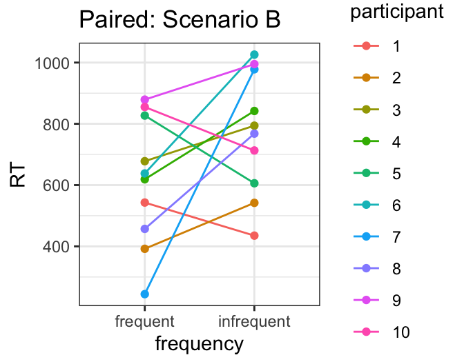
Participants in this experiment heard both frequent and infrequent words, introducing a participant-based dependency. The plots below show the same data as above, but coded for participant, so the paired participant data is linked by color (e.g. Participant 1’s data is shown in red). Scenarios A and B show two different possible participant parings. Would seeing the data in this way change your confidence about whether word frequency reliably influences RT? How would your confidence differ if you saw Scenario A vs. Scenario B?
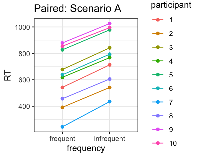
Let’s start with Scenario A. In this scenario, every single participant has higher RTs for infrequent than frequent words - which suggests that the frequency effect is very reliable, even if the effect size itself (the difference in RTs between frequent and infrequent words) is pretty small.
On the other hand, you would probably be less confident if you saw data that looked like Scenario B: some participants (e.g Participant 7) show large effects in the expected direction, but others show effects in the opposite direction: overall, there’s just a lot of individual variability. Given this, even though on average, RTs are shorter for frequent than for infrequent words, you might be less confident that the effect is reliable (note that as we have seen time and again in the past, increased variability lowers our confidence in the reliability of an effect!).
Statistical results
We can test for the significance of the difference between RTs of frequent vs. infrequent words using a linear model. Those we have looked at so far do not include any information about which datapoints belong to which participant, and in fact, the models we have used are based on the assumption that there is no pairing.
If we ignored this, and ran a simple linaer regression model on the data shown above, we would get a nonsignificant effect of frequency. However, if we change our model to incorporate information about the participant dependencies in the model (which we will see how to do below), we will get different results for Scenarios A and B. The estimates resulting from the three models are below. The models themselves are not shown.
| Model | Estimate (slope) | t-value | p-value | Effect of frequency significant? |
|---|---|---|---|---|
| Unpaired | 157 | 1.71 | 0.104 | No |
| Paired: Scenario A | 157 | 33.44 | < 0.001 | Yes |
| Paired: Scenario B | 157 | 1.75 | 0.114 | No |
First, notice that the Estimate (or slope) is the same for all models. This makes sense, because remember that this is just the average difference between the two levels…and the average difference is the same, no matter how the data is paired. However, the t- and p-values differ, indicating that the reliability of the effect differs. If the participants’ data is paired as in Scenario A, we see that the effect is highly reliable (high t-value, low p-value), whereas if participants’ data is paired as in Scenario B, the effect is not significant (low t-value, high p-value), matching our intuitions about how reliable the effect is in each scenario.
Furthermore, consider how failing to account for the dependencies in the model (i.e. using the Unpaired model) would affect the interpretation of the results in each scenario. If Scenario A was true, running the Unpaired model would result in a non-significant effect, even though there is one (a Type 2 error). On the other hand, if Scenario B was true, running the Unpaired model actually shows a more reliable effect (both are non-significant, but the p-value is smaller for the Unpaired model than the Scenario B paired model). In this case, running the Unpaired model artificially inflates the possibility of Type 1 error.
The purpose of this comparison is to demonstrate that including information about dependencies in the data can and does substantially affect results. It is critical that your model takes into account dependencies in the data; if not, the data is violating assumptions of the model and the inferences you are drawing from it not valid.
11.2 Mixed-effects regression model
The following example will walk through one case study dealing with participant-based dependencies. We will again be looking at Korean stops. Traditionally, the difference between aspirated and lenis stops is that aspirated have long VOT and lenis have short VOT. However, there is currently a merger going on, and we want to test whether there is still a VOT difference between lenis vs. aspirated VOT in younger speakers.
In past examples looking at Korean VOT, the data has been averaged so there is only one value per participant; however, the actual dataset has multiple words from each speaker. As you can see from the top of the dataset, there are multiple observations per participant (and multiple observations from each word; but we will ignore the item-based dependencies in this example for simplicity).
We will look at the question of whether VOT (outcome variable) differs for lenis vs. aspirated stops (predictor variable = stop type) in younger Seoul Korean speakers (the older speakers are not included in this dataset).
##   participant       VOT      type   word
## 1        S164  58.73382     lenis teoleo
## 2        S164 108.86829 aspirated  khani
## 3        S164  81.04599 aspirated  thaca
## 4        S164  31.07156     lenis  puleo
## 5        S164  53.72382     lenis   kaca
## 6 S164 96.73805 aspirated khani## participant VOT type
## S176 : 24 Min. : 16.58 aspirated:271
## S177 : 24 1st Qu.: 47.17 lenis :278
## S183 : 24 Median : 58.36
## S187 : 24 Mean : 60.91
## S167 : 23 3rd Qu.: 74.99
## S170 : 23 Max. :116.73
## (Other):407
## word
## tale : 50
## khani : 49
## teoleo : 49
## phali_arm: 48
## phulliph : 48
## thaca : 48
## (Other) :257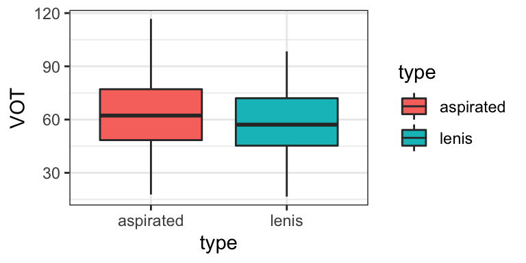
11.2.1 “Random effects” and “Mixed Effects Models”
In the model, we account for dependencies based on participant (or item) by incorporating what are often called “random effects.” There are two sub-types of random effects: “random intercepts” and “random slopes.” This allows your model to take into account patterns of (and make predictions for) specific participants. This allows for what otherwise would be considered random variation to be accounted for. The reason they are called “random” effects is because even though it models the behavior of each participant separately (e.g. P1 and P2 will each have their own predictions), you aren’t actually interested in knowing anything about these specific participants; instead, you are just recognizing the fact that there are different participants in your sample, with multiple observations, and incorporating the idea that individuals may show systematic behaviour.
Random effects contrast with fixed effects, which are the types of variables we’ve worked with so far. Mixed-effects models are those models that have both fixed and random effects.
11.2.2 Building the model
To incorporate information into the model:
- The relevant information needs to be coded in your dataset
- The structure of the model (the “formula” that goes into the command) needs to be modified to incorporate this information.
- We need to use a different command in R.
Encoding the relevant information
We can see that the relevant information (which participant said which word) is coded in the dataset in the participant column. We will call participant the “grouping” factor because we have different groups of data, one corresponding to each participant.
Building the model
When running a mixed-effects model in R, we need to use a different command, and for this we need to install and use the packages lme4 and lmerTest. We will then use the command lmer(formula, dataset) (which stands for linear mixed-effects regression). We can also use glmer() which is the mixed-model equivalent to glm() for categorical outcome variables. Just like in lm(), we will want to include a formula, followed by the relevant dataset.
The formula includes a mixture of fixed effects and random effects.
- The fixed effects component is exactly what we’re used to: outcome ~ predictor.
- The random effects component is added after this, in parentheses. It will be of the form (1 + (slope) | random factor), where random factor is the relevant random factor (here, participant).
- 1 is the intercept, and will always be included. This models a participant-specific intercept (average y-value) for each participant.
- There will also sometimes be a random slope. Whether or not this is included depends on the structure of your predictor variable(s). For each predictor, are the same participants involved in both of the levels? If so, you also need to include estimates for individual participant slopes. This is added into the random effects structure as follows: (1+predictor | participant).
| Random effects structure | When to use | Formula |
|---|---|---|
| none | no dependencies in the data | lm(outcome ~ predictor, data) |
| intercept only | multiple observations per participant; each participant in only one level of predictor | lmer(outcome ~ predictor + (1|participant), data) |
| intercept and slope | multiple observations per participant; each participant in both levels of predictor | lmer(outcome ~ predictor + (1+predictor|participant), data) |
Implementing and interpreting our example
In this case, where our outcome variable is VOT and our predictor is Stop Type, we will need to incorporate both random intercepts and slopes for participant, since there are multiple observations per participant, AND the same participants are producing both stop types (lenis and aspirated), so our random effects structure will be (1+type|participant). Note that if our predictor variable of interest was, for example, age, with levels Young and Old, we would not have the same participants in both levels, because you can’t be both young and old at the same time (OK, you can probably argue with that, but you know what I mean!). In this case, we would only have (1|participant) as the random effect structure.
Below is the command for building this model in R. Note that it doesn’t look that different except for the name of the command (lmer() vs. lm()) and the presence of the random effects structure.
## Linear mixed model fit by REML. t-tests use
##   Satterthwaite's method [lmerModLmerTest]
## Formula: VOT ~ type + (1 + type | participant)
##    Data: dat.kor
##
## REML criterion at convergence: 4610.9
##
## Scaled residuals:
##     Min      1Q  Median      3Q     Max
## -2.5536 -0.7019 -0.0246  0.6492  3.9156
##
## Random effects:
##  Groups      Name        Variance Std.Dev. Corr
##  participant (Intercept) 114.20   10.686
##              typelenis    97.65    9.882   -0.57
##  Residual                226.79   15.059
## Number of obs: 549, groups:  participant, 25
##
## Fixed effects:
##             Estimate Std. Error     df t value Pr(>|t|)
## (Intercept)   63.906      2.326 23.702   27.47   <2e-16 ***
## typelenis     -5.405      2.360 23.463   -2.29   0.0313 *
## ---
## Signif. codes:
## 0 '***' 0.001 '**' 0.01 '*' 0.05 '.' 0.1 ' ' 1
##
## Correlation of Fixed Effects:
##           (Intr)
## typelenis -0.590
Also, the interpretation is not much different than what you’re used to! You’ll see the coefficients table under “Fixed effects” (vs. random effects). You can also see information about the random effects above, but since we’re not so interested in the behavior of individuals in this case, we don’t have to worry about that!
As usual, we want to focus on our effect of interest, in this case the effect of Stop Type. We can see that the estimate is -5.405, indicating that lenis stops are on average about 5ms shorter in VOT than aspirated stops. The p-value of 0.03 indicates that this difference is significant. So even though it is tiny, these results provide evidence that there is still, on average, a difference between lenis and aspirated stop VOT in younger Korean speakers.
11.2.2.1 Summary
This is just a very basic introduction to the concepts underlying mixed-effects regression models. Since almost all linguistic research includes participant- and/or item-based dependencies, these are a commonly-used tool in linguistic research in real life, so it is well worth exploring further with other resources (e.g. Winter (2019), Chapter 14).
References
In an actual experiment testing this, we would likely have item-based dependencies as well, since the same words would likely be heard by all participants. However, we are ignoring this for now by considering the average RT for frequent words and the average RT for infrequent words for each participant, so there are no item-based dependencies in our analysis.↩︎