Chapter 8 Significance testing using linear models in R

In this section, we will show concretely how we can test the significance of relationships between variables: this encompasses a large range of the questions we want to ask when doing quantitative linguistic analysis! This will bring together the concepts of Null Hypothesis Statistical Testing (Chapter 7) and modeling relationships between variables as a line (Chapter 5).

Let’s return to our example of VOT of Korean aspirated stops. Let’s say we want to ask a question like:

Is there a significant correlation between VOT and age?
Does VOT differ significantly between older and younger speakers?
Is there a significant effect of age on VOT?

First, note that from a conceptual point of view, these three questions are asking the same thing! This becomes clear if we frame this in terms of an outcome variable (VOT) and a predictor variable (age): we want to know whether there is a systematic relationship between these two variables, or stated another way, is the value of the outcome variable (VOT) differs systematically depending on the value of the predictor variable (speakers’ age)?

Since our question of interest is whether VOT differs across ages, we will construct a null hypothesis that there is no difference in VOT across ages. Then we will test whether this null hypothesis is plausible for our data.

In the following sections, we will show how to test the significance of this relationship using linear models in R. We will show this in two ways: first, treating Age as a continuous variable, using speakers’ year of birth, and second, treating Age as a categorical variable, using a binary grouping of older vs. younger speakers. You will see that the logic of how this works is very similar whether you have a continuous or categorical predictor variable.

Review: Modeling relationships between variables as a line

Recall that the relationship between two variables can be modeled by finding the straight lines that best fit the data. We can do this for both continuous and categorical predictor variables. Remember that we can model a line with the formula \(y = \beta_1x+\beta_0\), where \(\beta_1\) is the slope.

a slope of zero indicates no relationship.
the larger the (absolute value of the) slope, the stronger the relationship.

The Korean data is plotted below, with VOT as the outcome variable and age as either continuous (by year of birth) or categorical variable (with speakers grouped into “older” or “younger” groups) as a predictor. Each point represents one speaker, and the best-fit regression line is included for each graph.

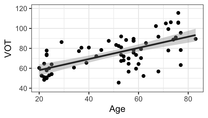
Regardless of whether we’re considering age as continuous or categorical, we see that in our sample, older speakers have longer VOT than younger speakers, on average. The evidence for this is that the best-fit regression line has a positive slope. What we want to do is test whether this relationship is meaningful, or significant.

8.1 Constructing the null and alternative hypotheses

We are interested in whether there is a significant relationship between VOT and age. Therefore, we will set up a null hypothesis that there is no significant relationship between VOT and age. In terms of the graphs, another way to state that there is no significant relationship is if the slope of the regression line is zero. Therefore, our null hypothesis is that the slope of the regression line is zero. The alternative hypothesis is that the slope of the regression line is not zero.

\[ H_0: slope = 0 \\ H_a: slope \neq 0 \] Now comes the inferential statistics, where we test the plausibility of the null hypothesis. It is possible to calculate a confidence interval for the slope of the regression line. R will do this for us - we don’t have to - but it takes into account the same ingredients as the CIs we calculated by hand for distributions of values: the sample slope itself, the variance, and the sample size. We then can simply look at whether 0 is within the 95% confidence interval for the slope. If it is not, we can reject the null hypothesis as implausible.

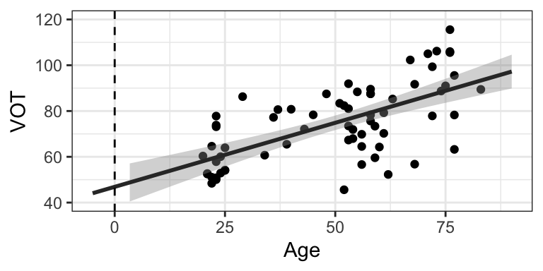
We’ll show how to get the CIs for slope automatically in the next section, but you can also see them on the graphs. In these graphs, you’ll see that there are grey bars surrounding the regression lines. These show the 95% confidence intervals for the slope. If the 95% confidence interval for the slope includes 0, you would be able to draw a straight horizontal line while remaining in the grey area. Since you can’t, this shows that 0 is not within the 95% confidence interval for (either of) these graphs.

8.2 Getting the numbers in R

To get the exact numbers, we use R to calculate the linear regression model that best fits the data. The linear regression model includes the best-fit regression line as well as the standard error, both of which are necessary to test the null hypothesis. We will walk through how to decode the output for two models, both testing the effect of age on VOT: the first will have age as a continuous variable and the second as a categorical variable. As you will see, the process and interpretation is very similar regardless of whether the predictor variable is continuous or categorical.

To create the linear model, we will use the lm(formula, dataset) function. The first argument is a formula in the form of y~x, where \(y\) is the outcome variable and \(x\) is the predictor variable. Both \(y\) and \(x\) need to be columns of a dataset; the name of the dataset is the second argument.

8.2.1 Linear regression with a continuous predictor

We will start by predicting VOT as a function of year of birth. The relevant columns in our dataset are VOT and yob, as shown in the first few lines of the dataset below.

## # A tibble: 6 × 5
## # Groups:   speaker, age, age.num [6]
##   age.num speaker   age ageGroup   VOT
##     <dbl> <chr>   <dbl> <fct>    <dbl>
## 1       1 S125       83 older     89.4
## 2       1 S126       77 older     95.5
## 3       1 S127       77 older     78.3
## 4       1 S128       76 older    106. 
## 5       1 S129       76 older    106. 
## 6       1 S130       76 older    116.

We will create an object called mdl, containing the linear model. We can then view the output of the model using the summary() function. There is a lot of information in the summary, but we will focus on the table under “Coefficients.” this will give us the most important information we need right now.

mdl.continuous = lm(VOT ~ age, dat.kor)
summary(mdl.continuous)

## 
## Call:
## lm(formula = VOT ~ age, data = dat.kor)
## 
## Residuals:
##      Min       1Q   Median       3Q      Max 
## -30.3739  -8.2438  -0.2538  10.2131  26.1451 
## 
## Coefficients:
##             Estimate Std. Error t value Pr(>|t|)    
## (Intercept) 46.88341    4.42549  10.594 8.54e-16 ***
## age          0.55945    0.08297   6.743 4.92e-09 ***
## ---
## Signif. codes:  0 '***' 0.001 '**' 0.01 '*' 0.05 '.' 0.1 ' ' 1
## 
## Residual standard error: 13.02 on 65 degrees of freedom
## Multiple R-squared:  0.4116, Adjusted R-squared:  0.4025 
## F-statistic: 45.47 on 1 and 65 DF,  p-value: 4.924e-09

Interpreting the coefficients

Let’s focus our attention on the table under “Coefficients.” There are two rows and 4 columns. The two rows correspond to the intercept and slope of the regression line. Remember, you can define a line with the formula \(y = \beta_1x+\beta_0\), where \(\beta_1\) is the slope and \(\beta_0\) is the y-intercept. The first row of the output gives information about the y-intercept \(\beta_0\), and the second (that starts with age) gives information about the slope \(\beta_1\), which in this case corresponds to the effect of age. The Estimate column provides the estimates for the formula for the line! If you just plug these in for your intercept and slope,you get the formula for the best-fit regression line. In this case, we can see that the formula for the best-fit regression line for the continuous data is as follows (rounded to 3 decimal places):

\[ y = \beta_1x + \beta_0 \\ y = 0.559x + 46.883 \]

##               Estimate Std. Error  t value     Pr(>|t|)
## (Intercept) 46.8834110 4.42549152 10.59394 8.539632e-16
## age          0.5594507 0.08296812  6.74296 4.923912e-09

Now let’s look at the rest of the numbers. For now, we will focus on the second row, the one corresponding to the slope. Here is the information we have.

Column	Description
`Estimate`	This provides the slope of the regression line. In other words, for every 1-unit increase in \(x\), the \(y\) value of the line will change by this amount. In this case, since age is coded in years, it means that for each additional year in age, VOT is higher by 0.559 ms.
`Std. Error`	This provides the standard error of the estimate. Remember that standard error is a measure of variance taking into account sample size.
`t value`	This gives the t-statistic. This is actually redundant, since \(t\) is simply the estimate divided by the standard error (\(0.5594507/0.08296812 = 6.7276\); you can test it out yourself!).
`Pr(>\|t\|)`	This is the p-value. It’s written in scientific notation: so another way to write this would be \(4.923912 * 10^{-9}\), or, by moving the decimal point left by 9, \(.000000004923912\). The column name refers to the fact that the p-value shows the probability that we would see an absolute value of \(t\) this large or higher under the null hypothesis that the slope is zero. In this case, the number is very small…meaning a very small probability!

So what do we actually need to get from this? Let’s return to our question. We are interested in testing the null hypothesis that there is no effect of age, in which case we would expect to find that the slope of the regression line is equal to zero. From our regression model, we can see the following information and make the following inferences. I have also included the plot below for reference.

The slope of the best-fit regression line for our sample data is positive (around \(0.559\)), showing that VOT increases as age increases, with a predicted average increase of 0.559ms per year.
The p-value is less than 0.05, indicating that it is highly improbable that we would see this extreme of a slope under the null hypothesis that the slope is zero.
Therefore, we can reject the null hypothesis that there is no effect of age, and conclude that there is a significant effect of age.
We won’t talk about the intercept here, but notice that the y-intercept (the place where the line passes the dotted vertical line) is between 40 and 50, corresponding to the exact estimate of \(46.883...\) shown in the coefficients table.

Making predictions

Since we know the estimated slope \(\beta_1\) and intercept for the regression line, and therefore the formula for the regression line, we can use this line to make predictions about the VOT (y-value) for a speaker of any age (x-value). All we have to do is plug in an age we want and we will get the predicted VOT. For example, we could substitute 80 for \(x\) in the equation below to find that the predicted VOT for a speaker of age 80 would be about 92 ms.

\[ y = 0.559x+ 46.883 \\ y = 0.559 \times 80 + 46.883 \\ y = 91.603 \]

8.2.2 Linear regression with a categorical predictor

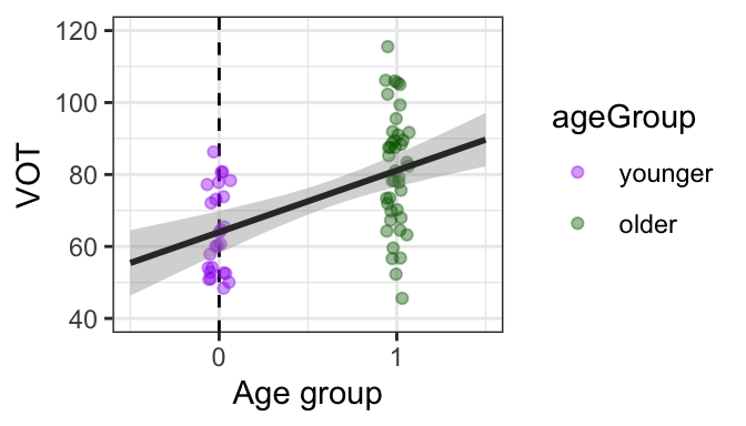
Now we will look at how to interpret the regression model when the predictor is categorical: in this case, looking at the data in terms of two age groups.

##               Estimate Std. Error   t value     Pr(>|t|)
## (Intercept)   63.99072   2.947883 21.707349 1.727067e-31
## ageGroupolder 17.13281   3.723257  4.601567 1.997205e-05

Again, in the Coefficients we see two lines, corresponding to the intercept and slope of the regression line. The interpretation is basically the same as above. The only additional information we need is to think about how to interpret the slope.

The estimate for the slope \(\beta_1\) is positive, around 17. In the case of a categorical predictor with two levels, as we have here, R will code them by default as 0 and 1, as we have. Because of this, a one-unit change in predictor is the difference between the two age groups. Since the slope corresponds to how much our outcome variables changes for each one-unit change in the predictor, a slope of around 17 means that there is a 17ms difference between older and younger groups. If you look back at the previous chapter, that’s exactly what we found!
Note that along with the name of the categorical variable (ageGroup), you also see “older.” This is because R has one level coded as the “reference level,” or the default level of the variable. In this case, the default level is “younger.” The presence of “older” in the output indicates that the slope is comparing the older group to the default “younger” group.
The p-value here is again very small (about 0.0000199). It is solidly below our threshold of .05. We can therefore reject the null hypothesis that zero is within the plausible range of slopes given our sample, and can say that the difference between groups is significant.
The estimate for the intercept, 63.99, is the value of y when x=0: you can confirm that this is where the regression line crosses the y-axis (dotted line). Since we’ve coded the younger group as zero, this is also the mean value for the younger group!

Interpretation of slope estimates (\(\beta_1\)) vs. p-values

It is tempting to think that you can judge the size of the effect based on the size of the p-value (with smaller p-values corresponding to larger effects). But this is not the case. The p-value is actually just a measure of how confident we can be that the null hypothesis is not true, given our data. The estimate itself is a better indicator of the magnitude of the effect.

8.2.3 Example: Two scenarios with the same slope/magnitude of effect

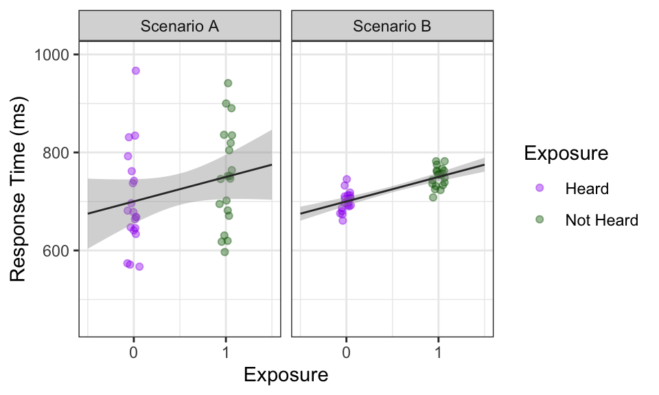
Consider the following two scenarios of (hypothetical) data showing response times of listeners to words that have been previously heard (0) or not previously heard (1).

dat %>% group_by(Exposure) %>% 
  summarize(rt=mean(rt))

## # A tibble: 2 × 2
##   Exposure     rt
##   <chr>     <dbl>
## 1 Heard       700
## 2 Not Heard   750

Based on the graphs and summary statistics below, we can see that in both scenarios, response times are on average 50 ms faster (lower) for words that have been heard. On the graphs, the slope is positive.

However, the data differs in how disperse it is, which ends up affecting the confidence intervals and our interpretation of the results:

There is greater variability in Scenario A than Scenario B.
The confidence intervals surrounding the lines in Scenario A are also much wider.
If you tried to draw a horizontal line through both of them, it would be possible in Scenario A, but not Scenario B.
Therefore, 0 is a plausible value for the slope in Scenario A, but not Scenario B.

8.2.3.1 Implementing the statistical test

Below is code for the two linear models in R, and the Coefficients section of the output. Remember that what we are primarily interested in is evaluating the slope, or the effect of Exposure. Therefore, we will be focusing on the second row in the output: that which corresponds to Exposure.

Model A

mdl.a = lm(rt ~ Exposure, filter(dat, scenario=="Scenario A"))
summary(mdl.a)$coef

##                   Estimate Std. Error   t value     Pr(>|t|)
## (Intercept)            700   22.36068 31.304952 9.676376e-29
## ExposureNot Heard       50   31.62278  1.581139 1.221352e-01

Model B

mdl.b = lm(rt ~ Exposure, filter(dat, scenario=="Scenario B"))
summary(mdl.b)$coef

##                   Estimate Std. Error    t value     Pr(>|t|)
## (Intercept)            700   4.472136 156.524758 5.229442e-55
## ExposureNot Heard       50   6.324555   7.905694 1.515962e-09

The Estimate corresponding to Exposure is the same for both models: 50. This is exactly what we expect. This shows that there is a 50 ms higher response time for Not-Heard items than for Heard items, just as we saw in the graphs.
The Standard error corresponding to Exposure is higher for Scenario A than Scenario B. This makes sense given what we saw in the graphs: there is a larger range of plausible values for the slope.
The p-value corresponding to Exposure is above the threshold of significance for Scenario A (p = 0.122) but below it for Scenario B (p < .001). This means:
- For Scenario A, we cannot reject the null hypothesis. We did not find sufficient evidence for a difference between groups.
- For Scenario B, we can reject the null hypothesis. We have found evidence for a significant difference between groups.

Although the two scenarios differ in whether they were significantly different (based on the p-value), the actual “size” of the effect in the sample – in other words, how much, on average, exposure affects reaction time – is exactly the same. It’s just our interpretation in the how confident we are in that effect that differs across the two scenarios.

8.3 Categorical predictors with more than two levels

When testing statistical differences between levels of a categorical predictor, remember that we are testing the null hypothesis that the difference between two levels is 0. So far, we have been dealing with categorical predictors with two levels. The estimate of the effect represents the difference between the mean values of the two levels, and our statistical test is used to determine whether that difference is plausibly zero. When dealing with categorical predictors of more than two levels, there are multiple possible 2-way comparisons to make, and our statistical model requires that we make a choice of which comparisons to test.

For a predictor variable with \(k\) levels, our statistical model allows us to make \(k-1\) comparisons. For a 2-level factor where \(k = 2\) (e.g. young vs. old), we therefore have one comparison, and since there’s only one comparison to make, there’s no issue. For a 3-level factor, (\(k = 3\) e.g. young vs. mid vs. old), there are potentially three comparisons: 1) young vs. old, 2) mid vs. old, and 3) young vs. mid. However, we can only test two of these.

One way to do this, and R’s default, is to set one level as the “reference level.” You can think of this as the level coded as 0. In this coding scheme, each of the non-reference levels is compared to the reference level. In our example of old vs. mid vs. young, if the reference level is “old,” then the two comparisons would be [mid vs. old] and [young vs. old]. The third possible comparison, [mid vs. young], would never be tested directly. This \(k-1\) limit in number of comparisons is a constraint of the statistical model; it is impossible to test all three in the same model. If you were particularly interested in the comparison of [mid vs. young], then it would make more sense to set either “mid” or “young” as the reference level. By default, R takes the first level alphabetically to be the reference level.

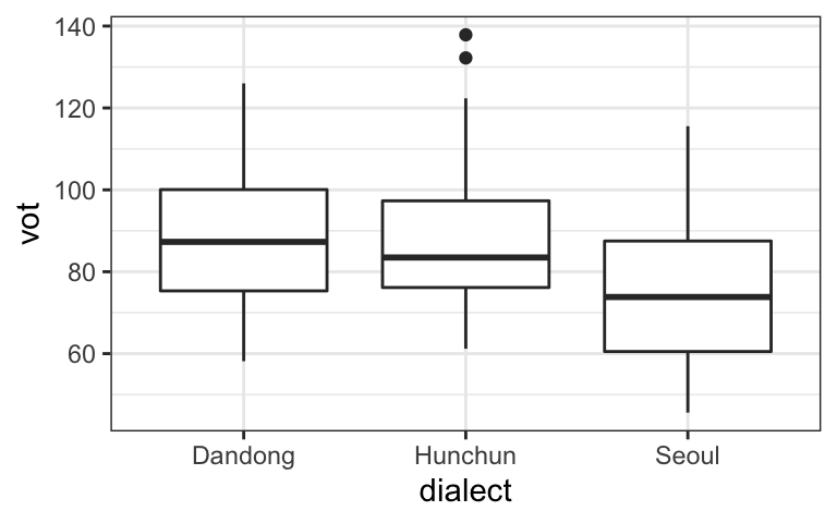
8.3.1 Example: comparison across 3 dialects

The following example shows data and a corresponding regression model examining how VOT differs across aspirated stops of three dialects of Korean. The boxplots in the graph indicate that Dandong and Hunchun look higher than Seoul. The graph also shows the levels with the reference level (Dandong) first.

## 
## Call:
## lm(formula = vot ~ dialect, data = dat.kor2)
## 
## Residuals:
##     Min      1Q  Median      3Q     Max 
## -30.306 -12.511  -1.471  11.800  50.089 
## 
## Coefficients:
##                Estimate Std. Error t value Pr(>|t|)    
## (Intercept)      88.456      2.126  41.612  < 2e-16 ***
## dialectHunchun   -0.681      3.056  -0.223    0.824    
## dialectSeoul    -13.725      2.972  -4.618 7.18e-06 ***
## ---
## Signif. codes:  0 '***' 0.001 '**' 0.01 '*' 0.05 '.' 0.1 ' ' 1
## 
## Residual standard error: 17.01 on 188 degrees of freedom
## Multiple R-squared:  0.1257, Adjusted R-squared:  0.1164 
## F-statistic: 13.52 on 2 and 188 DF,  p-value: 3.267e-06

When looking at the output of the corresponding regression model, we see three lines. The intercept shows the VOT when the predictor equals zero; in other words, the reference level: so Dandong speakers have an average VOT of 88.456 ms. There are two rows corresponding to the estimates for dialect, and each of them shows the difference between the dialect named in the row and the reference level. In other words, Hunchun speakers have on average -0.681 ms shorter VOT than Dandong speakers, and Seoul speakers have on average -13.725ms shorter VOT than Dandong speakers. The difference between Seoul and Dandong is significant, but the difference between Hunchun and Dandong is not.

Note that our model does not test the difference between Hunchun and Seoul. In order to do this, one of these two would have to be set as the reference level.

8.3.2 Changing the reference level

The choice of which level is the reference level does not make any difference in the overall “fit” of the model. Instead, it just makes a difference in terms of how the estimates are interpreted, and also which comparisons are tested statistically.

By default, R will set the order of levels alphabetically, so the first level alphabetically will be the reference level. If you want to change the reference level, you can do so manually as follows. The summary() of the column will show the order (the numbers below each level show the number of observations for each, which is not relevant for what we’re looking at right now; the order of the levels is what’s important!). The code below changes the reference level to Seoul.

## Dandong Hunchun   Seoul 
##      64      60      67

##   Seoul Dandong Hunchun 
##      67      64      60

Below is the output of the same model with this newly coded predictor.

## 
## Call:
## lm(formula = vot ~ dialect, data = dat.kor2)
## 
## Residuals:
##     Min      1Q  Median      3Q     Max 
## -30.306 -12.511  -1.471  11.800  50.089 
## 
## Coefficients:
##                Estimate Std. Error t value Pr(>|t|)    
## (Intercept)      74.731      2.078  35.969  < 2e-16 ***
## dialectDandong   13.725      2.972   4.618 7.18e-06 ***
## dialectHunchun   13.044      3.023   4.315 2.57e-05 ***
## ---
## Signif. codes:  0 '***' 0.001 '**' 0.01 '*' 0.05 '.' 0.1 ' ' 1
## 
## Residual standard error: 17.01 on 188 degrees of freedom
## Multiple R-squared:  0.1257, Adjusted R-squared:  0.1164 
## F-statistic: 13.52 on 2 and 188 DF,  p-value: 3.267e-06

In this model, the intercept (74.731) now reflects the mean VOT for Seoul speakers, with the two estimates corresponding to Dialect showing the difference of Dandong vs. Seoul and Hunchun vs. Seoul VOT, respectively. Both of these differences are significant.

8.3.3 Coding schemes

It can be tempting to want to test all possible comparisons, and you can do this by simply running multiple models with different reference levels, as we did above. However, it is not good practice to run multiple models on the same data, as it violates the assumptions underlying the inferential statistical method. Instead, it is better to think in advance of which comparisons are most important to test and set up the model such that you are able to test these relevant comparisons.

The choice of how to code levels of predictor variables is called the coding scheme. The method shown here, R’s default, is called dummy coding. However, there are many different coding schemes that can be used, and in practice, other coding schemes, such as sum coding or deviation coding, can be more generally useful. These are outside the scope of this course, but UCLA has an excellent reference for getting to know some of the other options.