Chapter 9 Categorical outcomes: Logistic regression

So far, we have dealt with outcome variables that are continuous (like VOT or response time or rating), and showed how to model the effect of predictor variables that are both continuous (like year of birth) or categorical (like younger vs. older age group).

This chapter shows how to deal with categorical outcome variables, focusing on outcome variables with 2 levels. A few examples of questions with a categorical outcome variable are given below. Note that the predictor variables can be either continuous or categorical.

Question	Outcome variable	Predictor variable
Does the frequency of use of ‘like’ as a discourse marker differ depending on the level of formality of speech style?	presence/absence of ‘like’	Formality
Does familiarity with a speaker influence listeners’ accuracy on a word memory task?	Accuracy	Familiarity with speaker
Does speakers’ choice between alternative lexical items (e.g. “You’re welcome” vs. “No worries” as a response to “Thank you”) differ based on the social status of their interlocutor?	Variant A vs. Variant B	Social status of interlocutor

In all of these cases, the outcome variable has one of two choices, which can be thought of as a binary choice between 0 and 1, just like a coin flip. Intuitively, what we want to know is if the probability of the outcome variable being 1 (vs. 0) differs for different values of the predictor variable. For example, in the example above, we might predict that participants are more likely to be accurate when they are familiar with the speaker.

Probabilities are bounded between 0 (corresponding to never) and 1 (corresponding to always). Because of the restricted space, it is not appropriate to model probabilities using linear regression (as will be demonstrated below). Instead, we will model what are called log odds, which is a logarithmic transformation of the probability space. You can convert from log odds to probability using the plogis(x) function, where x is log odds, and convert from probability to log odds using the formula log(p/(1-p)), where p is a probability:

Log odds to probability:

plogis(0)

## [1] 0.5

plogis(5)

## [1] 0.9933071

Probability to log odds:

log(.99/(1-.99))

## [1] 4.59512

The log odds space is not bounded: 0 log odds corresponds to 50% probability, with positive log odds corresponding to greater than 50% and negative corresponding to less than 50% probability. In order to model log odds, we will use what is called a logistic regression model.

Linear vs. logistic regression

From a practical point of view, using logistic regression instead of linear regression means:

a different formula in R
- Use the glm() (generalized linear model) function, and need to specify the argument “family=binomial”
different interpretation of the numbers in the model output.
- The model output is all in “log odds” space.
- Log odds are super non-intuitive.
- We generally want to interpret (and plot) things in terms of probabilities, which are more intuitive.

The choice between linear and logistic regression depends completely on whether the outcome variable is continuous vs. categorical. Both linear and logistic regression can have continuous or categorical predictor variables.

	Linear regression	Logistic regression
Response variable	Continuous	Binary (1 or 0)
Predictor variable	Continuous and/or categorical	Continuous and/or categorical
Intercept (\(\beta_{0}\))	Predicted value of \(y\) when \(X=0\)	Predicted log-odds of \(Y=1\) when \(X=0\)
Slope (\(\beta_{1}\))	Predicted change in \(y\) for one-unit change in \(x\)	Predicted change in log-odds of \(Y=1\) for a one-unit change in \(x\)

9.1 Logistic regression with continuous predictor

When someone says “Thank you” to you, what do you say? I’ve heard older people who are annoyed by the fact that younger people will say “No worries,” instead of “You’re welcome.” Let’s say you’re interested in how the choice of “no worries” vs. “you’re welcome” varies by age. You do an informal survey and ask people of different ages which they say. The (hypothetical) data is below. “No worries” is coded as 0, and “You’re welcome” as 1.

We can:

Plot the raw data (which will always be 0 for No Worries and 1 for You’re Welcome)
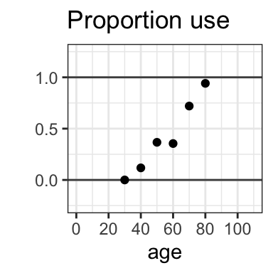
To make it easier to see the pattern, we can plot the proportional use of each variant across ages (below aggregated by decade): 0 = always uses No Worries, 1 = always uses You’re Welcome, .5 = half and half.
Based on this data, try to model the predicted probability of use of each variant across ages. A first thought might be to do this, as we did in the past, by trying to find a line that best fits the data. However, there is a problem with doing this. The possible probability space is bounded - probabilities can only go from 0 (never occurs) to 1 (always occurs). However, any non-horizontal line will always continue unbounded: you can’t make it stop at 0 and 1! In this case, the line predicts negative probabilities for a 10 year old, and probabilities greater than 1 for a 100 year old. We don’t want our model to be able to predict impossible values!
Our solution is that instead of trying to fit the probability space with a straight line via linear regression, we will model the predicted responses with logistic regression. The resulting model, when transformed and plotted in the probability space, will be an “s-curve” (or sigmoid curve, or logistic curve) which is bounded by 0 and 1.

9.1.1 Running the model

In the graphs above, we can see that the proportion use of “You’re Welcome” (vs. “No worries”) as a response to “Thank you” is higher for older than for younger speakers. We can use a logistic regression model, using the glm() function in R, to test whether this relationship between age and choice of variant is significant.

First, let’s look at the data. Each row has a participant, their age, the variant they chose, and a column variant.num that codes You’re Welcome as 1 and No worries as 0. We will want to use this binary variable as our response variable.

##   participant age        variant variant.num
## 1          S1  35     No worries           0
## 2          S2  62     No worries           0
## 3          S3  72 You're welcome           1
## 4          S4  35     No worries           0
## 5          S5  76 You're welcome           1
## 6          S6  51 You're welcome           1

Now we will run the model and view the summary. Note that we use a function with the following form: glm(y ~ x, dataset, family=binomial) This is similar to the lm() function we used for linear models. The structure for the formula for the model is the same: \(y\) is the response variable (in this case, variant.num) and \(x\) is the predictor (in this case age). You also need to include the argument family=binomial to tell it to be modeling a binomial distribution.

## 
## Call:
## glm(formula = variant.num ~ age, family = binomial, data = dat.thanks)
## 
## Deviance Residuals: 
##     Min       1Q   Median       3Q      Max  
## -1.9343  -0.7342  -0.3764   0.7540   2.3162  
## 
## Coefficients:
##             Estimate Std. Error z value Pr(>|z|)    
## (Intercept)  -6.2073     1.0110  -6.140 8.25e-10 ***
## age           0.1027     0.0171   6.009 1.87e-09 ***
## ---
## Signif. codes:  0 '***' 0.001 '**' 0.01 '*' 0.05 '.' 0.1 ' ' 1
## 
## (Dispersion parameter for binomial family taken to be 1)
## 
##     Null deviance: 201.90  on 149  degrees of freedom
## Residual deviance: 148.72  on 148  degrees of freedom
## AIC: 152.72
## 
## Number of Fisher Scoring iterations: 4

As before, we will mainly be paying attention to the coefficients of the model. The estimate for the second row, corresponding to age, is again going to be the slope of the best-fit line. However, the model has been working in log-odds space, so this estimate tells you that there is a 0.1027 predicted change in log odds of a “you’re welcome” response for every one-unit increase in age. For now, you can just focus on the fact that this is a positive value. Positive log odds mean increased probability, so this estimate shows (as we saw in the graph), that the probability of a you’re welcome response increases with age. The other columns of the coefficient table are the same, though in this case a z-statistic replaces the earlier t-statistic. However, it serves a similar function: larger z-values indicate a more reliable effect. The last column contains the p-value; as this number is very small, we can say that the effect of age on choice of variant is significant.

Basically, we will rely on the model to test the direction of the effect (in this case, more “you’re welcome” corresponding to older age) and whether it is significant. You can then use the proportion responses in the data to give a more intuitive sense of how big this effect is. In this example, as is shown in the graph, it’s a pretty big effect. Based on the graphs and our model outcome, we can conclude: There is a significant age-based difference in preference for “You’re Welcome” vs. “No Worries” as a response to “Thank you”: younger speakers almost always choose “No worries,” while older speakers almost always choose “You’re welcome.”

9.2 Logistic regression with categorical predictor

Below, we’ll look at the example of Labov’s famous department store experiment. Labov tested whether salespeople from New York City department stores catering to different social classes showed different use of a phonological variable: presence or absence of coda ‘r’ in words like ‘car’ and ‘birth.’ He went into the stores and asked salespeople about a product that he knew would be on the fourth floor, and he noted whether for each of these words, they used a rhotic version (fourth, floor) or a nonrhotic version (fou’th, floo’).

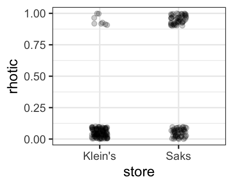
Below are data from two different department stores: Saks (more expensive) and Klein’s (less expensive). Our outcome variable is the choice of variant: rhotic (coded as 1) or nonrhotic (coded as 0). The predictor variable is Store, with levels Sak’s and Klein’s.

First, we will plot the data. As above, plotting the raw data is a bit difficult to interpret because all observations are either 1 or 0. Instead, plotting the average for each store is more informative. This shows clearly that there is greater use of the rhotic forms (the prestige forms) at Saks than at Klein’s.

We can then use a logistic regression model to test whether this is significant.

## 
## Call:
## glm(formula = rhotic ~ store, family = binomial, data = dat.labov)
## 
## Deviance Residuals: 
##     Min       1Q   Median       3Q      Max  
## -1.1345  -0.4523  -0.4523   1.2209   2.1591  
## 
## Coefficients:
##             Estimate Std. Error z value Pr(>|z|)    
## (Intercept)  -2.2285     0.2296  -9.704  < 2e-16 ***
## storeSaks     2.1267     0.2746   7.745 9.53e-15 ***
## ---
## Signif. codes:  0 '***' 0.001 '**' 0.01 '*' 0.05 '.' 0.1 ' ' 1
## 
## (Dispersion parameter for binomial family taken to be 1)
## 
##     Null deviance: 456.22  on 392  degrees of freedom
## Residual deviance: 382.70  on 391  degrees of freedom
## AIC: 386.7
## 
## Number of Fisher Scoring iterations: 4

In this case, examining the coefficients, we see that the estimate corresponding to our predictor variable is positive (2.1267). This means that there is a 2.12 log odds increase in use of rhotic forms for Saks as compared to Klein’s, and the small p-value indicates that there is a significant difference in usage across the two stores.

In terms of interpreting the actual values, remember that the intercept indicates the value (in log odds) of the outcome variable when the predictor is zero, and the estimate for the slope indicates how much the log odds of the outcome changes for every one-unit increase in the predictor. In this case the “0-coded” level of the predictor variable is Klein’s. Therefore, -2.2285 is the log odds of a rhotic form at Klein’s, and to find the log odds of a rhotic form at Saks, you just need to add the estimate for the slope: -2.2285 + 2.1267 = -0.1018. We can convert these values to probabilites using the plogis() function, to find that the predicted probability of a rhotic form at each of the stores (9.7% at Klein’s and 47.5% at Saks):

plogis(-2.2285)

## [1] 0.09722021

plogis(-0.1018)

## [1] 0.474572

While it’s possible to get the exact values by converting the log odds back to probabilities, as above, another way to interpret the results in a more intuitive way, we can return to our graphs, and also calculate the mean proportions for each store, to conclude the following: The use of rhotic (vs. non-rhotic) forms was found to be greater in speakers working at Saks (47.5% use of rhotic forms) than in speakers working at Klein’s (9.7% use of rhotic forms), and this difference is significant.

## # A tibble: 2 × 2
##   store   rhotic
##   <chr>    <dbl>
## 1 Klein's 0.0972
## 2 Saks    0.475